| Oracle® Communications Data Model Implementation and Operations Guide Release 11.3.1 Part Number E28442-04 |
|
|
PDF · Mobi · ePub |
| Oracle® Communications Data Model Implementation and Operations Guide Release 11.3.1 Part Number E28442-04 |
|
|
PDF · Mobi · ePub |
This chapter provides information about creating reports, queries, and dashboards against the data in a Oracle Communications Data Model warehouse. It contains the following topics:
Troubleshooting Oracle Communications Data Model Report Performance
Tutorial: Creating a New Oracle Communications Data Model Dashboard
Tutorial: Creating a New Oracle Communications Data Model Report
There are two main approaches to creating reports from data in an Oracle Communications Data Model warehouse:
With relational reporting, you create reports against the analytical layer entities using the fact entities as the center of the star with the reference entities (that is, DWR_ and DWL_ tables) acting as the dimensions of the star. Typically the fact entities include the derived and aggregate entities (that is, DWD_ and DWA_ tables). However in some cases, you may need to use the base entities (that is, DWB_ tables) along with the reference tables to generate more detailed reports.
The reference tables (that is, DWR_ tables) typically represent dimensions which contain a business hierarchy and are present in the form of snowflake entities containing a table for each level of the hierarchy. This allows us to attach the appropriate set of reference entities for the multiple subject area and fact entities composed of differing granularity.
For example, you can use the set of tables comprising DWR_DAY as well as DWR_BSNS_MO, DWR_BSNS_QTR, DWR_BSNS_YR tables to query against a DAY level CDR Wireless entity such as DWD_VOI_CALL_DAY. On the other hand, you need to use the higher level snowflakes at Month level and above such as DWR_BSNS_MO, DWR_BSNS_QTR, DWR_BSNS_YR in order to query against the MONTH level CDR Wireless entity such as DWA_VOI_CALL_MO.
The lookup tables (that is tables, with the DWL_ prefix) represent the simpler dimensions comprising a single level containing a flat list of values. Typically, most reporting tools add a superficial top level to the dimension. These could be individual tables starting with DWL_ or views (also named DWL_) on DWL_CODE_MASTER that break out different code types into separate dimensions.
With OLAP reporting, you access Oracle OLAP cubes using SQL against the dimension and cube (fact) views. Cubes and dimensions are represented using a star schema design. Dimension views form a constellation around the cube (or fact) view. The dimension and cube views are relational views with names ending with _VIEW. Typically, the dimension view used in the reports is named dimension_hierarchy_VIEW and the cube view is named cube_VIEW.
Unlike the corresponding relational dimension entities stored in DWR_ tables, the OLAP dimension views contains information relating to the whole dimension including all the levels of the hierarchy logically partitioned on the basis of a level column (identified as level_name). On a similar note, the cube views also contain the facts pertaining to the cross-combination of the levels of individual dimensions which are part of the cube definition. Also the join from the cube view and the dimension views are based on the dimension keys along with required dimension level filters.
Although the OLAP views are also modeled as a star schema, there are certain unique features to the OLAP reporting methodology which requires special modeling techniques in Oracle Business Intelligence Suite Enterprise Edition.
See also:
The Oracle By Example tutorial, entitled "Using Oracle OLAP 11g With Oracle BI Enterprise Edition". To access the tutorial, open the Oracle Learning Library in your browser by following the instructions in "Oracle Technology Network"; and, then, search for the tutorials by name.The rest of this chapter explains how to create Oracle Communications Data Model reports. For examples of Oracle Communications Data Model reports, see:
"Tutorial: Creating a New Oracle Communications Data Model Dashboard"
"Tutorial: Creating a New Oracle Communications Data Model Report"
The sample reports provided with Oracle Communications Data Model that are documented in Oracle Communications Data Model Reference.
Sample reports and dashboards are delivered with Oracle Communications Data Model. These sample reports illustrate the analytic capabilities provided with Oracle Communications Data Model -- including the OLAP and data mining capabilities.
See:
Oracle Communications Data Model Installation Guide for more information on installing the sample reports and deploying the Oracle Communications Data Model RPD and webcat on the Business Intelligence Suite Enterprise Edition instance.The sample reports were developed using Oracle Business Intelligence Suite Enterprise Edition which is a comprehensive suite of enterprise business intelligence products that delivers a full range of analysis and reporting capabilities. Thus, the reports also illustrate the ease with which you can use Oracle Business Intelligence Suite Enterprise Edition Answers and Dashboard presentation tools to create useful reports.
You can use Oracle Business Intelligence Suite Enterprise Edition Answers and Dashboard presentation tools to customize the predefined sample dashboard reports:
Oracle BI Answers. Provides end user ad hoc capabilities in a pure Web architecture. Users interact with a logical view of the information -- completely hidden from data structure complexity while simultaneously preventing runaway queries. Users can easily create charts, pivot tables, reports, and visually appealing dashboards.
Oracle BI Interactive Dashboards. Provide any knowledge worker with intuitive, interactive access to information. The end user can be working with live reports, prompts, charts, tables, pivot tables, graphics, and tickers. The user has full capability for drilling, navigating, modifying, and interacting with these results.
See:
Oracle Communications Data Model Reference for detailed information on the sample reports.The ocdm_sys schema defines the relational tables and views in Oracle Communications Data Model. You can use any SQL reporting tool to query and report on these tables and views.
Oracle Communications Data Model also supports On Line Analytic processing (OLAP) reporting using OLAP cubes defined in the ocdm_sys schema. You can query and write reports on OLAP cubes by using SQL tools to query the views that are defined for the cubes or by using OLAP tools to directly query the OLAP components.
See also:
"Reporting Approaches in Oracle Communications Data Model", "Oracle OLAP Cube Views", and the discussion on querying dimensional objects in Oracle OLAP User's Guide.Example 5-1 Creating a Relational Query for Oracle Communications Data Model
For example, assume that you want to know the total call minutes for the top ten customers in the San Francisco area for March 2009. To answer this question, you might have to query the tables described in the following table.
| Entity Name | Table Name | Description |
|---|---|---|
| WIRELESS CALL EVENT | DWB_WRLS_CALL_EVT |
Occurrences of the wireless call. |
| CUSTOMER | DWR_CUST |
Individual customers |
| ADDRESS LOCATION | DWR_ADDR_LOC |
All addresses. The table has levels as country, state, city, address, and so on. |
| GEOGRAPHY CITY | DWR_GEO_CITY |
The CITY level of the GEOGRAPHY hierarchy. |
To perform this query, you execute the following SQL statement.
SELECT cust_key, tot_call_min FROM
(select         round(sum(call.call_drtn)/60,2) tot_call_min , call.cust_key
from    DWB_WRLS_CALL_EVT call,
DWR_CUST     cust,
DWR_ADDR_LOC addr,
DWR_GEO_CITY city
         Where to_date(to_char(call.evt_begin_dt,'MON-YY'),'MON-YY') like        to_date('MAR-09','MON-YY')
and cust.cust_key = call.cust_key
and cust.addr_loc_key = addr.addr_loc_key
and addr.geo_city_key = city.geo_city_key
and initcap(city.geo_city_name)='San Francisco'
group by call.cust_key
order by 1 desc) WHERE ROWNUM < 10;
The result of this query is shown below.
CUST_KEY TOT_CALL_MIN
---------- ------------
      3390        101.6
      4304       100.25
      4269        97.37
      4152        93.02
      4230        92.97
      4157        92.95
      3345        91.62
      4115        48.43
      4111        44.48
A typical query in the access layer is a join between the fact table and some number of dimension tables and is often referred to as a star query. In a star query each dimension table is joined to the fact table using a primary key to foreign key join. Normally the dimension tables do not join to each other.
Typically, in this kind of query all of the WHERE clause predicates are on the dimension tables and the fact table. Optimizing this type of query is very straight forward.
To optimize this query, do the following:
Create a bitmap index on each of the foreign key columns in the fact table or tables
Set the initialization parameter STAR_TRANSFORMATION_ENABLED to TRUE.
This enables the optimizer feature for star queries which is off by default for backward compatibility.
If your environment meets these two criteria, your star queries should use a powerful optimization technique that rewrites or transforms your SQL called star transformation. Star transformation executes the query in two phases:
Retrieves the necessary rows from the fact table (row set).
Joins this row set to the dimension tables.
The rows from the fact table are retrieved by using bitmap joins between the bitmap indexes on all of the foreign key columns. The end user never needs to know any of the details of STAR_TRANSFORMATION, as the optimizer automatically chooses STAR_TRANSFORMATION when it is appropriate.
Example 5-2, "Star Transformation" gives the step by step process to use STAR_TRANSFORMATION to optimize a star query.
Example 5-2 Star Transformation
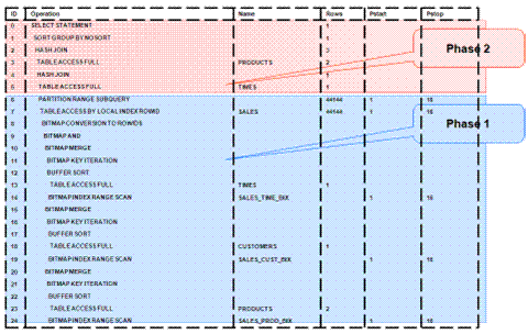
A business question that could be asked against the star schema in Figure 3-1, "Star Schema Diagram" would be "What was the total number of umbrellas sold in Boston during the month of May 2008?"
The original query.
select SUM(quantity_sold) total_umbrellas_sold_in_Boston
From Sales s, Customers c, Products p, Times t
Where s.cust_id=cust_id
And s.prod_id = p.prod_id
And s.time_id=t.time_id
And c.cust_city='BOSTON'
And p.product='UMBRELLA'
And t.month='MAY'
And t.year=2008;
As you can see all of the where clause predicates are on the dimension tables and the fact table (Sales) is joined to each of the dimensions using their foreign key, primary key relationship.
Take the following actions:
Create a bitmap index on each of the foreign key columns in the fact table or tables.
Set the initialization parameter STAR_TRANSFORMATION_ENABLED to TRUE.
The rewritten query. Oracle rewrites and transfers the query to retrieve only the necessary rows from the fact table using bitmap indexes on the foreign key columns
select SUM(quantity_sold
From Sales
Where cust_id IN
(select c.cust_id From Customers c Where c.cust_city='BOSTON')
And s.prod_id IN
(select p.prod_id From Products p Where  p.product='UMBRELLA')
And s.time_id IN
(select t.time_id From Times(Where t.month='MAY' And tyear=2008);
By rewriting the query in this fashion you can now leverage the strengths of bitmap indexes. Bitmap indexes provide set based processing within the database, allowing you to use various fact methods for set operations such as AND, OR, MINUS, and COUNT. So, you use the bitmap index on time_id to identify the set of rows in the fact table corresponding to sales in May 2008. In the bitmap the set of rows are actually represented as a string of 1's and 0's. A similar bitmap is retrieved for the fact table rows corresponding to the sale of umbrellas and another is accessed for sales made in Boston. At this point there are three bitmaps, each representing a set of rows in the fact table that satisfy an individual dimension constraint. The three bitmaps are then combined using a bitmap AND operation and this newly created final bitmap is used to extract the rows from the fact table needed to evaluate the query.
Using the rewritten query, Oracle joins the rows from fact tables to the dimension tables.
The join back to the dimension tables is normally done using a hash join, but the Oracle Optimizer selects the most efficient join method depending on the size of the dimension tables.
The following figure shows the typical execution plan for a star query when STAR_TRANSFORMATION has kicked in. The execution plan may not look exactly as you expected. There is no join back to the customer table after the rows have been successfully retrieved from the Sales table. If you look closely at the select list, you can see that there is not anything actually selected from the Customers table so the optimizer knows not to bother joining back to that dimension table. You may also notice that for some queries even if STAR_TRANSFORMATION does kick in it may not use all of the bitmap indexes on the fact table. The optimizer decides how many of the bitmap indexes are required to retrieve the necessary rows from the fact table. If an additional bitmap index would not improve the selectivity, the optimizer does not use it. The only time you see the dimension table that corresponds to the excluded bitmap in the execution plan is during the second phase or the join back phase.
Take the following actions to identify problems generating a report created using Oracle Business Intelligence Suite Enterprise Edition:
In the (Online) Oracle BI Administrator Tool, select Manage, then Security, then Users, and then ocdm.
Ensure that the value for Logging level is 7.
Open the Oracle Communications Data Model Repository, select Manage, and then Cache.
In the right-hand pane of the Cache Manager window, select all of the records, then right-click and select Purge.
Run the report or query that you want to track using the SQL log.
Open the query log file (NQQuery.log) under OracleBI\server\Log.
The last query SQL is the log of the report you have just run. If an error was returned in your last accessed report, there is an error at the end of this log.
The following examples illustrate how to use these error messages:
Example 5-3, "Troubleshooting an Oracle Communications Data Model Report"
Example 5-4, "Troubleshooting a Report: A Table Does Not Exist"
Example 5-5, "Troubleshooting a Report: When the Database is Not Connected"
Example 5-3 Troubleshooting an Oracle Communications Data Model Report
Assume the log file contains the following error.
Query Status: Query Failed: [nQSError: 15018] Incorrectly defined logical table source (for fact table Customer Mining) does not contain mapping for [Customer.Cell Phone Number, Customer.Customer Segment Name, Customer.Party Name].
This error occurs when there is a problem in the Business layer in your Oracle Business Intelligence Suite Enterprise Edition repository.
In this case, you need to check the mapping for Customer.Cell Phone Number, Customer.Customer Segment Name, and Customer.Party Name.
Example 5-4 Troubleshooting a Report: A Table Does Not Exist
Assume the log file contains the following error.
Query Status: Query Failed: [encloser: 17001] Oracle Error code: 942, message: ORA-00942: table or view does not exist.
This error occurs when the physical layer in your Oracle Business Intelligence Suite Enterprise Edition repository has the table which actually does not exist in the Database.
To find out which table has problem:
Copy the SQL query to database environment.
Execute the query.
The table which does not exist is marked out by the database client.
Example 5-5 Troubleshooting a Report: When the Database is Not Connected
Assume the log file contains the following error.
Error: Query Status: Query Failed: [nQSError: 17001] Oracle Error code: 12545, message: ORA-12545: connect failed because target host or object does not exist.
Meaning: This error occurs when the Database is not connected.
Action: Check connecting information in physical layer and ODBC connection to ensure that the repository is connecting to the correct database.
Two common query techniques are "as is" and "as was" queries:
An As Is query has the following characteristics:
The resulting report shows the data as it happened.
The snowflake dimension tables are also joined using the surrogate key columns (that is the primary key and foreign key columns).
The fact table is joined with the dimension tables (at leaf level) using the surrogate key column.
Slowly-changing data in the dimensions are joined with their corresponding fact records and are presented individually.
It is possible to add up the components if the different versions share similar characteristics.
An As Was query (also known as point-in-time analysis) has the following characteristics:
The resulting report shows the data that would result from freezing the dimensions and dimension hierarchy at a specific point in time.
Each snowflake table is initially filtered by applying a point-in-time date filter which selects the records or versions which are valid as of the analysis date. This structure is called the point-in-time version of the snowflake.
The filtered snowflake is joined with an unfiltered version of itself by using the natural key. All of the snowflake attributes are taken from the point-in-time version alias. The resulting structure is called the composite snowflake.
A composite dimension is formed by joining the individual snowflakes on the surrogate key.
The fact table is joined with the composite dimension table at the leaf level using the surrogate key column.
The point-in-time version is super-imposed on all other possible SCD versions of the same business entity -- both backward as well as forward in time. Joining in this fashion gives the impression that the dimension is composed of only the specific point-in-time records.
All of the fact components for various versions add up correctly due to the super-imposition of point-in-time attributes within the dimensions.
Based on the Data used for the examples, the following examples illustrate the characteristics of As Is and As Was queries:
Example 5-6, "As Is Query for Tax Collection Split by Marital Status"
Example 5-7, "As Was Queries for Tax Collection Split by Marital Status"
Example 5-8, "As Is Query for Tax Collection Data Split by County"
Example 5-9, "As Was Queries for Tax Collection Data Split by County"
Assume that your data warehouse has a Customer table, a County, and a TaxPaid fact table. As of January 1, 2011, these tables include the values shown below.
Customer Table
| Cust Id | Cust Cd | Cust Nm | Gender | M Status | County Id | County Cd | Country Nm | ... | Eff Frm | Eff To |
|---|---|---|---|---|---|---|---|---|---|---|
| 101 | JoD | John Doe | Male | Single | 5001 | SV | Sunnyvale | ... | 1-Jan-11 | 31-Dec-99 |
| 102 | JaD | Jane Doe | Female | Single | 5001 | SV | Sunnyvale | ... | 1-Jan-11 | 31-Dec-99 |
| 103 | JiD | Jim Doe | Male | Married | 5002 | CU | Cupertino | ... | 1-Jan-11 | 31-Dec-99 |
County Table
| County Id | County CD | County Nm | Population | ... | Eff Frm | Eff To |
|---|---|---|---|---|---|---|
| 5001 | SV | Sunnyvale | Very High | ... | 1-Jan-11 | 31-Dec-99 |
| 5002 | CU | Cupertino | High | ... | 1-Jan-11 | 31-Dec-99 |
TaxPaid Table
| Cust Id | Day | Tax Type | Tax |
|---|---|---|---|
| 101 | 1-Jan-11 | Professional Tax | 100 |
| 102 | 1-Jan-11 | Professional Tax | 100 |
| 103 | 1-Jan-11 | Professional Tax | 100 |
Assume that the following events occurred in January 2011:
On January 20, 2011, Jane Doe marries.
On Jan 29, 2011, John Doe moves from Sunnyvale to Cupertino.
Consequently, as shown below, on February 1, 2011, the Customer and TaxPaid tables have new data while the values in the County table stay the same.
Customer table
| Cust Id | Cust Cd | Cust Nm | Gender | M Status | County Id | County Cd | Country Nm | ... | Eff Frm | Eff To |
|---|---|---|---|---|---|---|---|---|---|---|
| 101 | JoD | John Doe | Male | Single | 5001 | SV | Sunnyvale | ... | 1-Jan-11 | 29-Jan-11 |
| 102 | JaD | Jane Doe | Female | Single | 5001 | SV | Sunnyvale | ... | 1-Jan-11 | 20-Jan-11 |
| 103 | JiD | Jim Doe | Male | Married | 5002 | CU | Cupertino | ... | 1-Jan-11 | 31-Dec-99 |
| 104 | JaD | Jane Doe | Female | Married | 5001 | SV | Sunnyvale | ... | 21-Jan-11 | 31-Dec-99 |
| 105 | JoD | John Doe | Male | Single | 5002 | CD | Cupertino | ... | 30-Jan-11 | 31-Dec-99 |
County table
| County Id | County CD | County Nm | Population | ... | Eff Frm | Eff To |
|---|---|---|---|---|---|---|
| 5001 | SV | Sunnyvale | Very High | ... | 1-Jan-11 | 31-Dec-99 |
| 5002 | CU | Cupertino | High | ... | 1-Jan-11 | 31-Dec-99 |
TaxPaid Table
| Cust Id | Day | Tax Type | Tax |
|---|---|---|---|
| 101 | 1-Jan-11 | Professional Tax | 100 |
| 102 | 1-Jan-11 | Professional Tax | 100 |
| 103 | 1-Jan-11 | Professional Tax | 100 |
| 105 | 1-Feb-11 | Professional Tax | 100 |
| 104 | 1-Feb-11 | Professional Tax | 100 |
| 103 | 1-Feb-11 | Professional Tax | 100 |
Example 5-6 As Is Query for Tax Collection Split by Marital Status
Assuming the Data used for the examples, to show the tax collection data split by martial status, the following SQL statement that joins the TaxPaid fact table and the Customer dimension table on the cust_id surrogate key and the Customer and County snowflakes on the cnty_id surrogate key.
SELECT cust.cust_nm, cust.m_status, SUM(fct.tx)
FROM taxpaid fct, customer cust, county cnty
WHERE fct.cust_id = cust.cust_id
AND cust.cnty_id = cnt.cnt_id
GROUP BY cust.cust_nm, cust.m_status
ORDER BY 1,2,3;
The results of this query are shown below. Note that there are two rows for Jane Doe; one row for a marital status of Married and another for a marital status of Single.
| Cust Nm | M Status | Tax |
|---|---|---|
| Jane Doe | Married | 100 |
| Jane Doe | Single | 100 |
| Jim Doe | Married | 200 |
| John Doe | Single | 200 |
Example 5-7 As Was Queries for Tax Collection Split by Marital Status
Assuming the Data used for the examples, issue the following SQL statement to show the tax collection data split by marital status using an analysis date of January 15, 2011.
select
   cust.cust_nm, cust.m_status, sum(fct.tax)
from
   TaxPaid fct,
   (
      select
         cust_act.cust_id, cust_pit.cust_cd, cust_pit.cust_nm,
         cust_pit.m_status, cust_pit.gender,
         cust_pit.cnty_id, cust_pit.cnty_cd, cust_pit.cnty_nm
      from Customer cust_act
      inner join (
         select
            cust_id, cust_cd, cust_nm,
            m_status, gender,
            cnty_id, cnty_cd, cnty_nm
         from Customer cust_all
         where to_date('15-JAN-2011', 'DD-MON-YYYY') between eff_from and eff_to
      ) cust_pit
      on (cust_act.cust_cd = cust_pit.cust_cd)
   ) cust,
   (
      select
         cnty_act.cnty_id, cnty_pit.cnty_cd, cnty_pit.cnty_nm
      from County cnty_act
      inner join (
         select
            cnty_id, cnty_cd, cnty_nm
         from County cnty_all
         where to_date('15-JAN-2011', 'DD-MON-YYYY') between eff_from and eff_to
      ) cnty_pit
      on (cnty_act.cnty_cd = cnty_pit.cnty_cd)
   ) cnty
where fct.cust_id = cust.cust_id
and cust.cnty_id = cnty.cnty_id
GROUP BY cust.cust_nm, cust.m_status
order by 1,2,3;
The results of this query are shown below. Since Jane Doe was single on January 15, 2011 (the analysis date), all tax for Jane Doe is accounted under her Single status.
| Cust Nm | M Status | Tax |
|---|---|---|
| Jane Doe | Single | 200 |
| Jim Doe | Married | 200 |
| John Doe | Single | 200 |
Assume instead that you issued the exact same query except that for the to_date phrase you specify 09-FEB-2011 rather than 15-JAN-2011. Since Jane Doe was married on February 9, 2011, then, as shown below all tax for Jane Doe would be accounted under her Married status.
| Cust Nm | M Status | Tax |
|---|---|---|
| Jane Doe | Married | 200 |
| Jim Doe | Married | 200 |
| John Doe | Single | 200 |
Example 5-8 As Is Query for Tax Collection Data Split by County
Assuming the Data used for the examples, issue the following SQL statement to show the tax collection data split by county.
SELECT cust.cust_nm, cnty.cnty_nm, SUM(fct.tax)
FROM TaxPaid fct, customer cust, county cnty
WHERE fct.cust_id = cust.cust_id
AND cust.cnty_id = cnty.cnty_ID
GROUP BY cut.cust_nm, cnty.cnty_nm
ORDER BY 1,2,3;
The results of this query are shown below. Note that since John Doe lived in two different counties, there are two rows of data for John Doe.
| Cust Nm | County Nm | Tax |
|---|---|---|
| Jane Doe | Sunnyvale | 200 |
| Jim Doe | Cupertino | 200 |
| John Doe | Cupertino | 100 |
| John Doe | Sunnyvale | 100 |
Example 5-9 As Was Queries for Tax Collection Data Split by County
Assuming the Data used for the examples, issue the following SQL statement to show the tax collection data split by county using an analysis date of January 15, 2011.
select
   cust.cust_nm, cnty.cnty_nm, sum(fct.tax)
from
  TaxPaid fct,
   (
      select
         cust_act.cust_id, cust_pit.cust_cd, cust_pit.cust_nm,
         cust_pit.m_status, cust_pit.gender,
         cust_pit.cnty_id, cust_pit.cnty_cd, cust_pit.cnty_nm
      from Customer cust_act
      inner join (
         select
            cust_id, cust_cd, cust_nm,
            m_status, gender,
            cnty_id, cnty_cd, cnty_nm
         from Customer cust_all
         where to_date('15-JAN-2011', 'DD-MON-YYYY') between eff_from and eff_to
      ) cust_pit
      on (cust_act.cust_cd = cust_pit.cust_cd
   ) cust,
   (
      select
         cnty_act.cnty_id, cnty_pit.cnty_cd, cnty_pit.cnty_nm
      from County cnty_act
      inner join (
         select
            cnty_id, cnty_cd, cnty_nm
         from County cnty_all
         where to_date('15-JAN-2011', 'DD-MON-YYYY') between eff_from and eff_to
      ) cnty_pit
      on (cnty_act.cnty_cd = cnty_pit.cnty_cd)
   ) cnty
where fct.cust_id = cust.cust_id
and cust.cnty_id = cnty.cnty_id
GROUP BY cust.cust_nm, cnty.cnty_nm
order by 1,2,3;
The results of this query are shown below. Note that since John Doe was in Sunnyvale as of the analysis date of January 15, 2011, all tax for John Doe is accounted for under the Sunnyvale county.
| Cust Nm | County Nm | Tax |
|---|---|---|
| Jane Doe | Sunnyvale | 200 |
| Jim Doe | Cupertino | 200 |
| John Doe | Sunnyvale | 200 |
Assume instead that you issued the exact same query except that for the to_date phrase you specify 09-FEB-2011 rather than 15-JAN-2011. Since John Doe lived in Cupertino on February 9, 2011, then, as shown below all tax for John Doe would be accounted under Cupertino.
| Cust Nm | County Nm | Tax |
|---|---|---|
| Jane Doe | Sunnyvale | 200 |
| Jim Doe | Cupertino | 200 |
| John Doe | Cupertino | 200 |
This tutorial explains how to create a new dashboard based on the Oracle Communications Data Model webcat included with the sample Oracle Business Intelligence Suite Enterprise Edition reports delivered with Oracle Communications Data Model.
See:
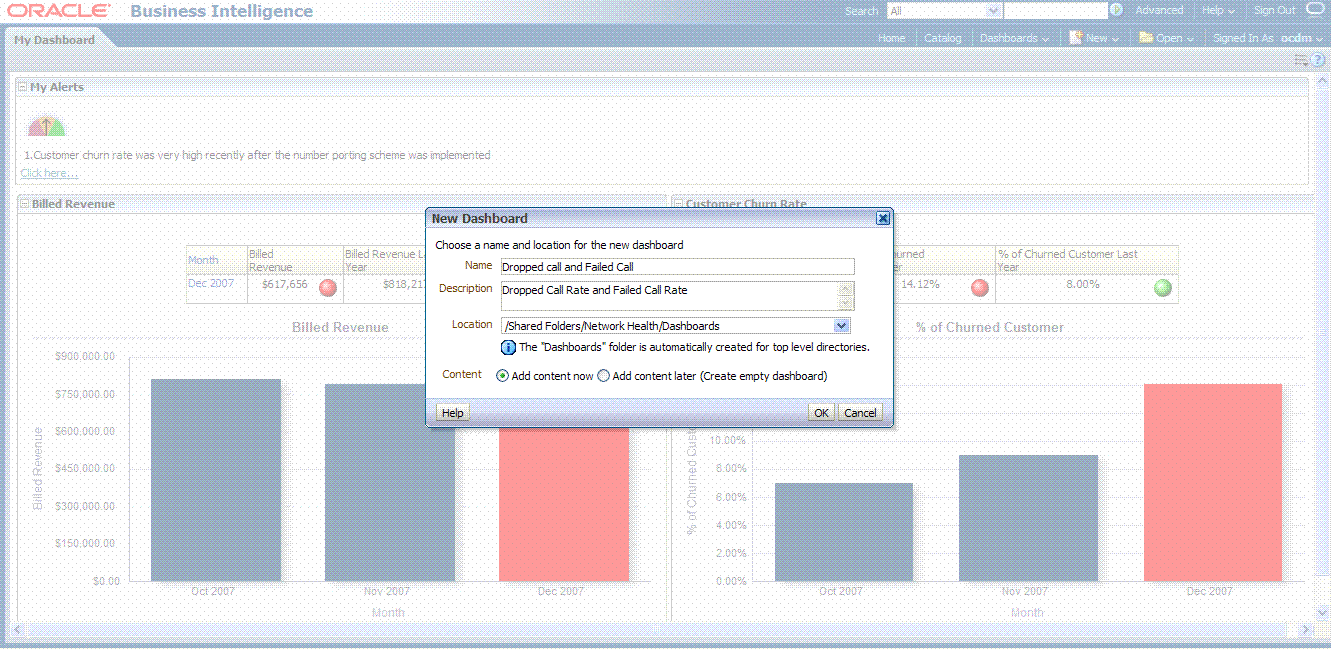
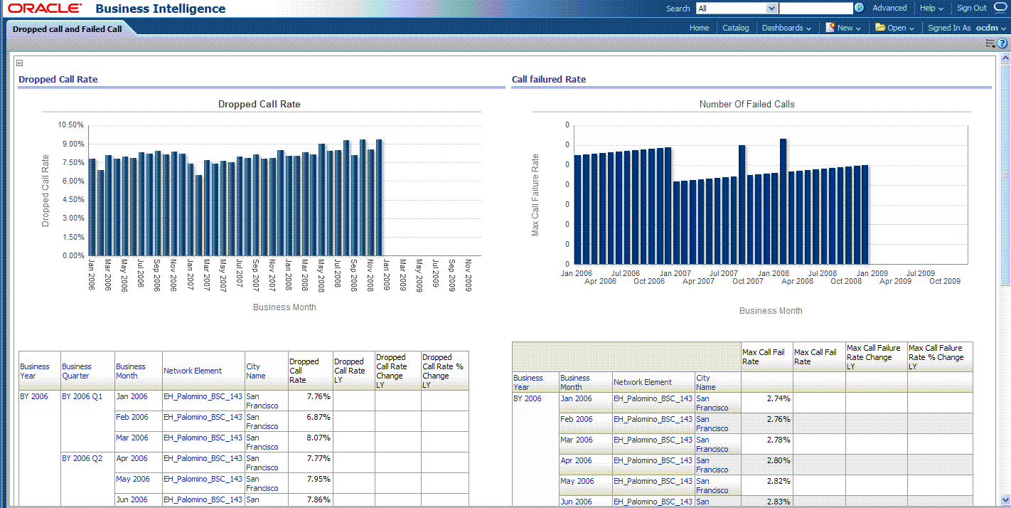
Oracle Communications Data Model Installation Guide for more information on installing the sample reports and deploying the Oracle Communications Data Model RPD and webcat on the Business Intelligence Suite Enterprise Edition instance.In this example assume that you want to create a dashboard named "Dropped call and Failed Call", and put both "Dropped Call Rate Report" and "Failed Call Rate Report" into this new dashboard.
To create a dashboard, take the following steps:
In the browser, open the login page at http://servername:9704/analytics where servername is the server on which the webcat is installed.
Login with username of ocdm, and provide the password.
Then, click newDashboard to create an Oracle Business Intelligence Suite Enterprise Edition dashboard.
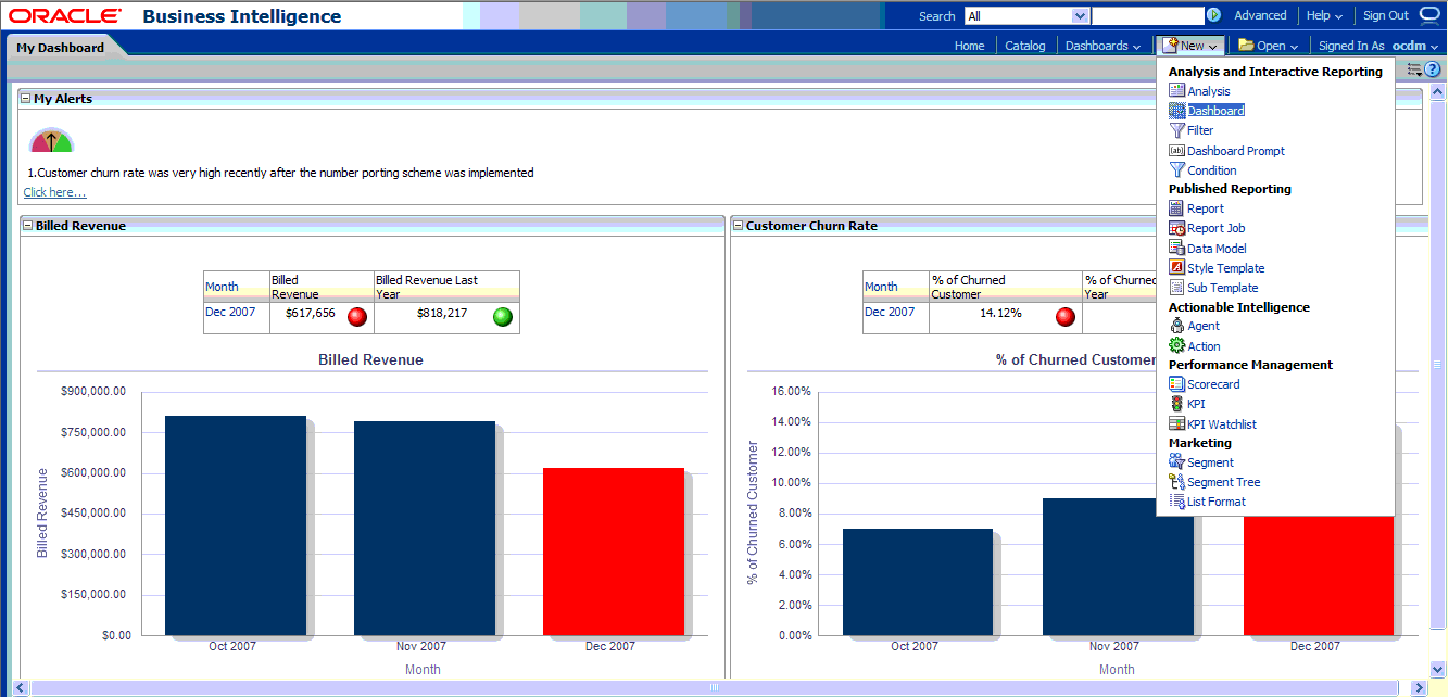
Input name and description, save it to the Network Health folder. Click OK.
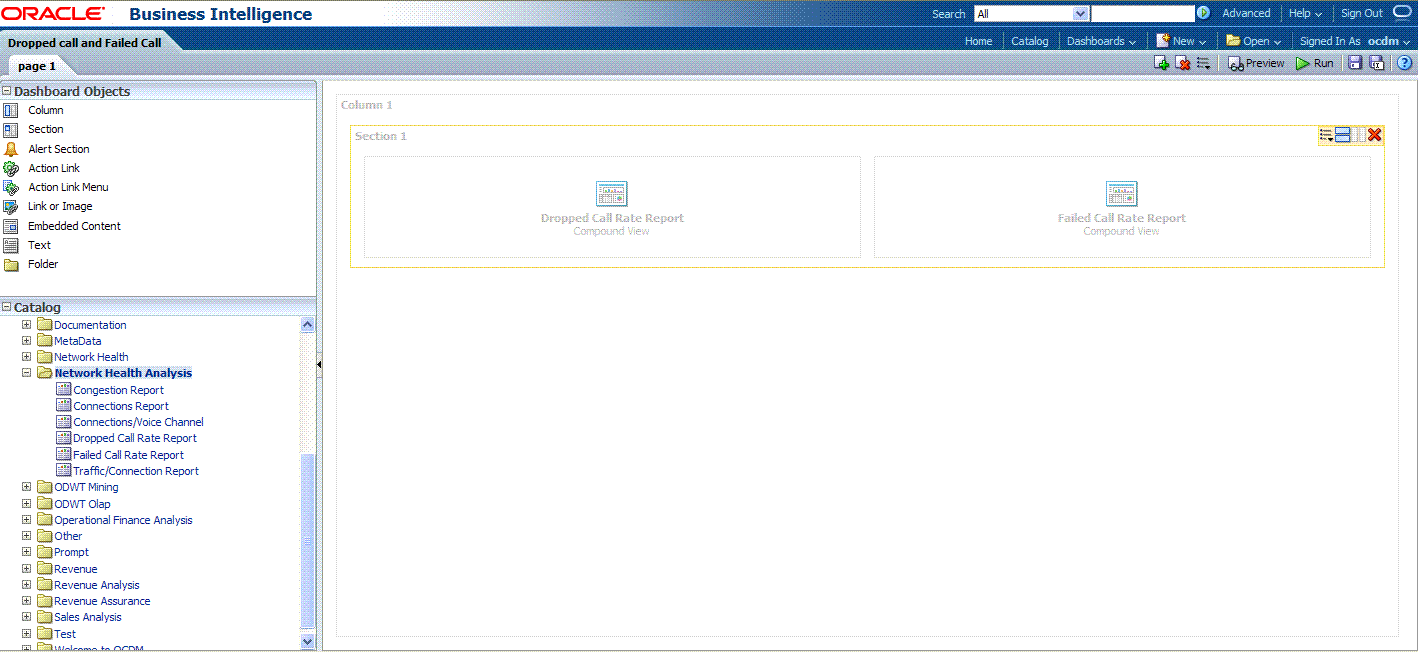
In the Catalog view, expand the Network Health Analysis folder. You can see the Failed Call Rate Report and Dropped Call Rate Report.
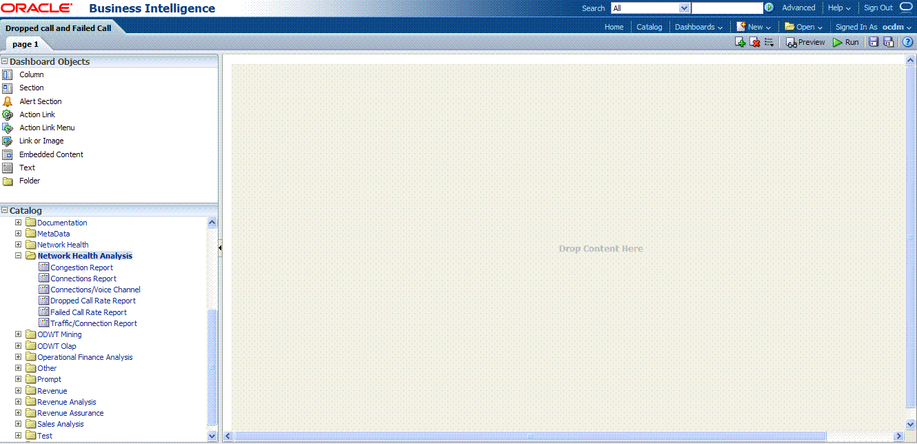
Drag the Failed Call Rate Report and Dropped Call Rate Report from the Catalog view into the right panel.
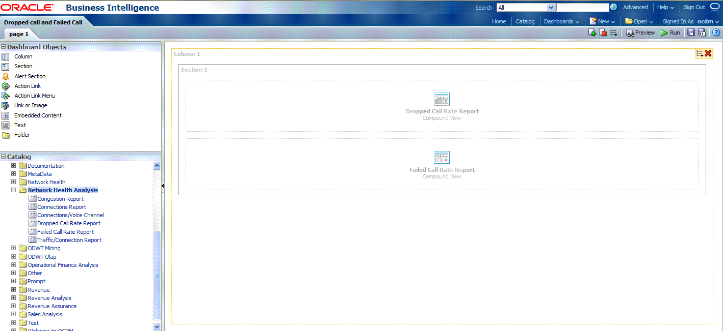
You can change the layout of this section to organize the two reports by horizontal or vertical.
Note that the page name is still "Page1" so you must change it.
To change the page name:
Select the Dashboard.
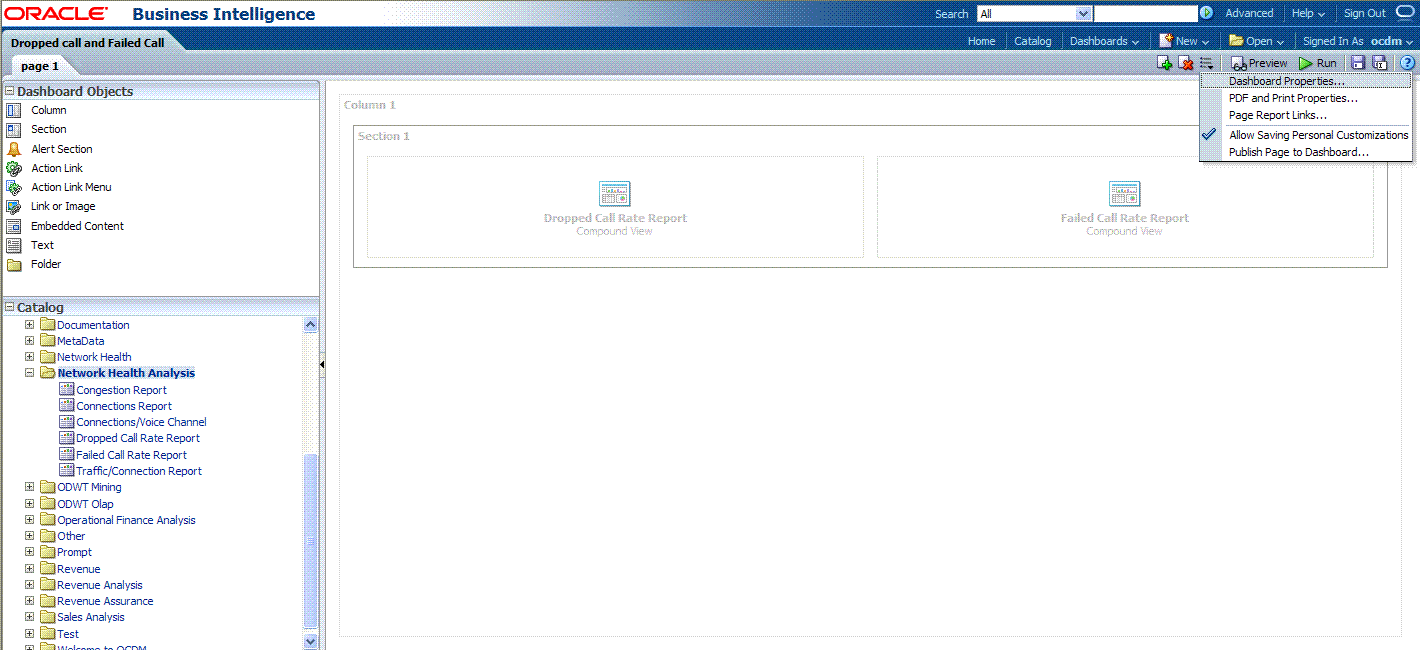
In Dashboard Properties window, click Change Name.
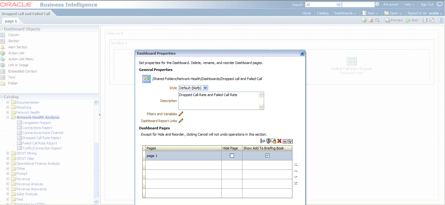
Change the name to "Dropped Call Rate and Failed Call Rate", then click OK.
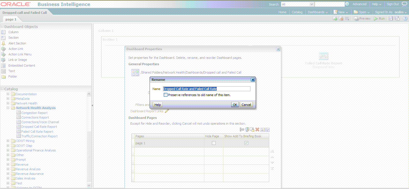
Click Save on the top of the dashboard. Now you have a new dashboard.
Oracle by Example:
For more information on creating dashboards see the "Creating Analyses and Dashboards 11g" OBE tutorial.To access the tutorial, open the Oracle Learning Library in your browser by following the instructions in "Oracle Technology Network"; and, then, search for the tutorial by name.
This tutorial explains how to create a new report based on the Oracle Communications Data Model webcat included with the sample Oracle Business Intelligence Suite Enterprise Edition reports delivered with Oracle Communications Data Model.
See:
Oracle Communications Data Model Installation Guide for more information on installing the sample reports and deploying the Oracle Communications Data Model RPD and webcat on the Business Intelligence Suite Enterprise Edition instance.In this example, assume that you want to create a report named "Dropped call vs. Failed Call" to put both dropped call rate and failed call rate in one report.
To create a this new report, take the following steps:
In the browser, open the login page at http://servername:9704/analytics where servername is the server on which the webcat is installed.
Login with username of ocdm, and provide the password.
Then, click newAnalysis to create an Oracle Business Intelligence Suite Enterprise Edition report.
Select Subject Area, then select ODWT to create a relational report. 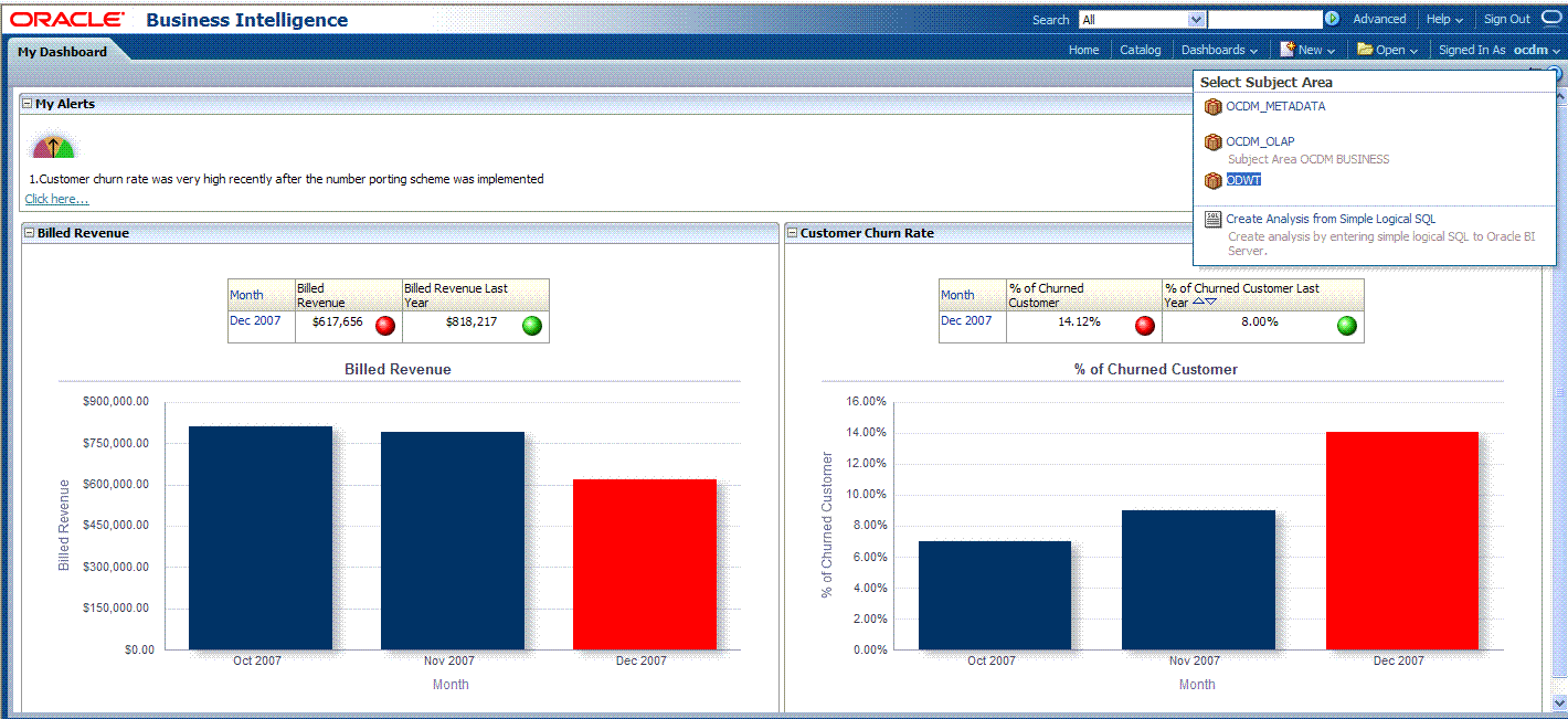
Description of the illustration rpt2.gif
Drag and put the dimension and fact columns into the Select Columns panel. 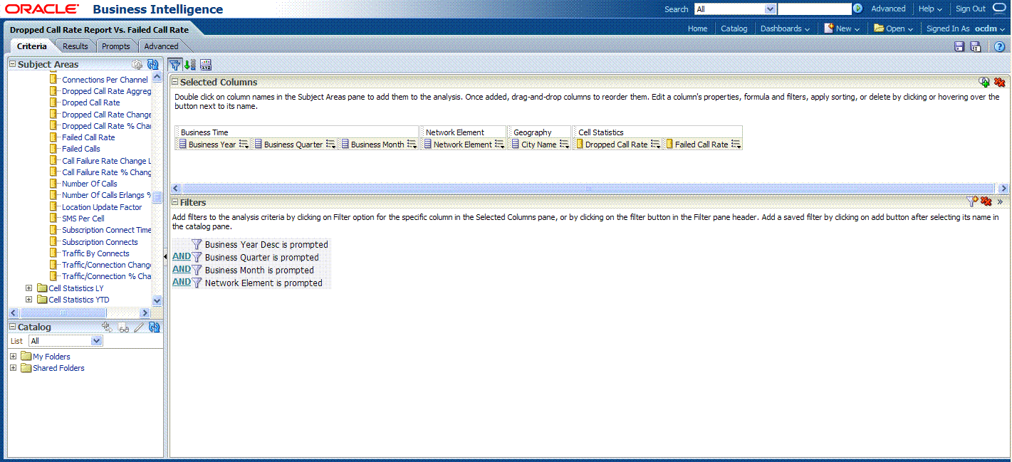
Description of the illustration rpt3.gif
Select the Results tab to view the report 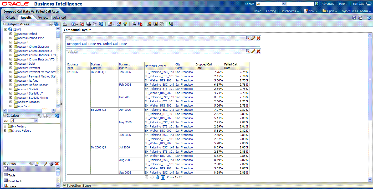
Description of the illustration rpt4.gif
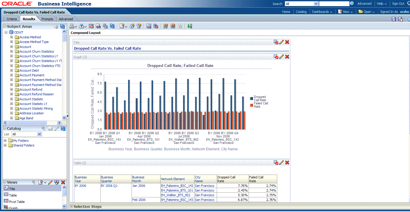
Click New View to add a chart into report. 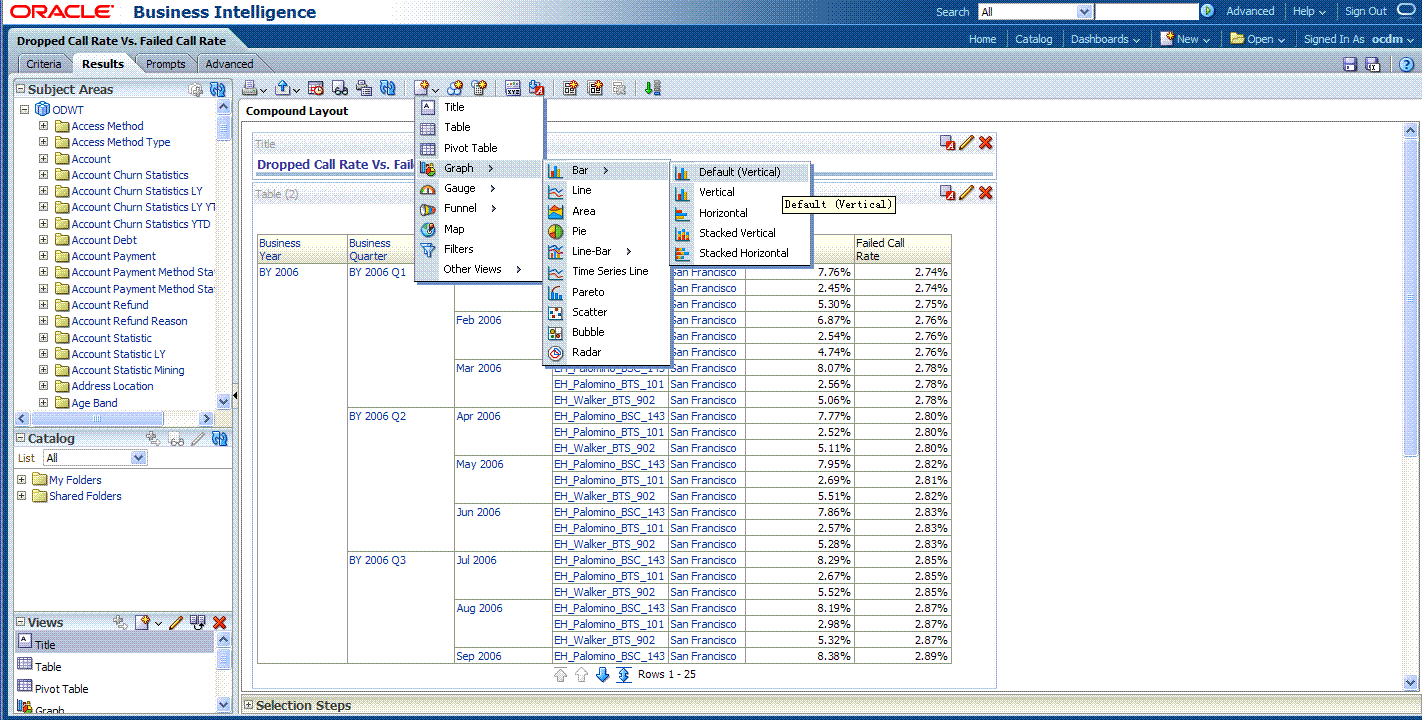
Description of the illustration rpt5.gif
Click Save to save this report to the Network Health Analysis folder
Oracle by Example:
For more information on creating a report, see the "Creating Analyses and Dashboards 11g" OBE tutorial.To access the tutorial, open the Oracle Learning Library in your browser by following the instructions in "Oracle Technology Network"; and, then, search for the tutorial by name.
|
Copyright © 2011, 2012, Oracle and/or its affiliates. All rights reserved. Legal Notices |
|