| Oracle® Retail Data Model Implementation and Operations Guide Release 11.3.1 Part Number E20363-02 |
|
|
PDF · Mobi · ePub |
| Oracle® Retail Data Model Implementation and Operations Guide Release 11.3.1 Part Number E20363-02 |
|
|
PDF · Mobi · ePub |
This chapter provides general information about customizing the physical model of Oracle Retail Data Model and more detailed information about customizing the foundation layer of the physical model. This chapter contains the following topics:
See also:
Chapter 3, "Access Layer Customization"The default physical model of Oracle Retail Data Model defines:
Over 1,250 tables and 18,500 attributes
Over 1,800 industry measures and KPIs
12 pre-built data mining models
30 OLAP dimensions and 28 pre-built OLAP cubes
The default physical model of Oracle Retail Data Model shares characteristics of a multischema "traditional" data warehouse, as described in "Layers in a "Traditional" Data Warehouse", but defines all data structures in a single schema as described in "Layers in the Default Oracle Retail Data Model Warehouse".
Layers in a "Traditional" Data Warehouse
Historically, three layers are defined for a data warehouse environment:
Staging layer. This layer is used when moving data from the transactional system and other data sources into the data warehouse itself. It consists of temporary loading structures and rejected data. Having a staging layer enables the speedy extraction, transformation and loading (ETL) of data from your operational systems into data warehouse without disturbing any of the business users. It is in this layer the much of the complex data transformation and data quality processing occurs. The most basic approach for the design of the staging layer is as a schema identical to the one that exists in the source operational system.
Note:
In some implementations this layer is not necessary, because all data transformation processing is done "on the fly" as data is extracted from the source system before it is inserted directly into the foundation layer.Foundation or integration layer. This layer is traditionally implemented as a Third Normal Form (3NF) schema. A 3NF schema is a neutral schema design independent of any application, and typically has a large number of tables. It preserves a detailed record of each transaction without any data redundancy and allows for rich encoding of attributes and all relationships between data elements. Users typically require a solid understanding of the data to navigate the more elaborate structure reliably. In this layer data begins to take shape and it is not uncommon to have some end-user application access data from this layer especially if they are time sensitive, as data becomes available here before it is transformed into the Access and Performance layer.
Access layer. This layer is traditionally defined as a snowflake or star schema that describes a "flattened" or dimensional view of the data.
Layers in the Default Oracle Retail Data Model Warehouse
Oracle Retail Data Model warehouse environment also consists of three layers, as shown in Figure 2-1. Note, in the Oracle Retail Data Model the definitions of the foundation and access layers are combined in a single schema.
Figure 2-1 Layers of an Oracle Retail Data Model Warehouse
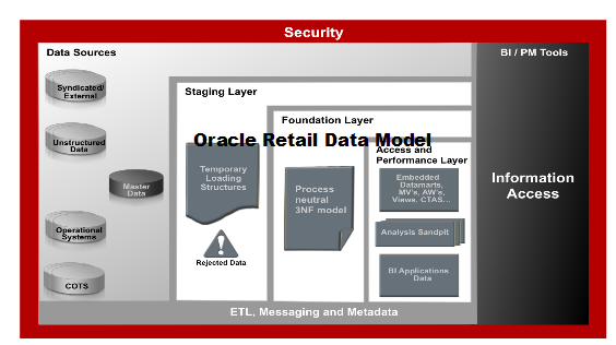
The layers in the Oracle Retail Data Model warehouse are:
Staging layer. As in a "traditional" data warehouse environment, an Oracle Retail Data Model warehouse environment can have a staging layer. See the Oracle Retail Data Model Release Notes for more details on the staging layer.
Foundation and Access layers. The physical objects for these layers are defined in a single schema, the ordm_sys schema:
Foundation layer. The foundation layer of the Oracle Retail Data Model is defined by base (DWB_) and Reference (DWR_) tables that present the data in 3NF; this layer also includes the lookup and control tables defined in the ordm_sys schema (that is, the tables that have the DWL_ and DWC_ prefixes).
Access layer. The Access layer of Oracle Retail Data Model is defined by derived and aggregate tables (defined with DWD_ and DWA_ prefixes), cubes (defined with a CB$ prefix), and views (that is, views defined with the _VIEW suffix). These structures provide a summarized or "flattened" perspective of the data in the foundation layer.
This layer also contains the results of the data mining models which are stored in derived (DWD_) tables.
The starting point for the Oracle Retail Data Model physical data model is the 3NF logical data model. The physical data model mirrors the logical model as much as possible, although some changes in the structure of the tables or columns may be necessary, and defines database objects (such as tables, cubes, and views).
To customize the default physical model of Oracle Retail Data Model take the following steps:
Answer the questions outlined in "Questions to Answer Before You Customize the Physical Model".
Familiarize yourself with the characteristics of the logical and physical model of Oracle Retail Data Model as outlined in"Characteristics of the Default Physical Model" and presented in detail in Oracle Retail Data Model Reference.
Modify the foundation level of your physical model of Oracle Retail Data Model, as needed. See "Common Change Scenarios When Customizing the Foundation Layer of Oracle Retail Data Model" for a discussion of when customization might be necessary.
When defining physical structures:
Keep the foundation layer in 3NF form.
Use the information presented in "General Recommendations When Designing Physical Structures" to guide you when designing the physical objects.
Follow the conventions used when creating the default physical model of Oracle Retail Data Model as outlined in "Conventions When Customizing the Physical Model".
Tip:
Package the changes you make to the physical data model as a patch to theordm_sys schema.Modify the access layer of your physical model of Oracle Retail Data Model as discussed in Chapter 3, "Access Layer Customization".
When designing the physical model, remember that the logical data model is not one-to-one with the physical data model. Consider the load, query, and maintenance requirements when you are designing the physical model customizations. For example, answer the following questions before you design the physical data model:
Identify the scope of the changes. See "Common Change Scenarios When Customizing the Foundation Layer of Oracle Retail Data Model" for an overview discussion of making physical data model changes when your business needs do not result in a logical model that is the same as the Oracle Retail Data Model logical model.
What is the result of the source data profile?
What is the data load frequency for each table?
How many large tables are there and which tables are these?
How will the tables and columns be accessed? What are the common joins?
What is your data backup strategy?
When developing the physical model for Oracle Retail Data Model, the following conventions were used. Continue to follow these conventions as you customize the physical model.
General Naming Conventions for Physical Objects
Follow these guidelines for naming physical objects that you define:
When naming the physical objects follow the naming guidelines for naming objects within an Oracle Database schema. For example:
Table and column names must start with a letter, can use only 30 alphanumeric characters or less, cannot contain spaces or some special characters such as "!" and cannot use reserved words.
Table names must be unique within a schema that is shared with views and synonyms.
Column names must be unique within a table.
Although it is common to use abbreviations in the physical modeling stage, as much as possible, use names for the physical objects that correspond to the names of the entities in the logical model. Use consistent abbreviations to avoid programmer and user confusion.
When naming columns, use short names if possible. Short column names reduce the time required for SQL command parsing.
The ordm_sys schema delivered with Oracle Retail Data Model uses the prefixes and suffixes shown in the following table to identify object types.
| Prefix or Suffix | Used for Name of These Objects |
|---|---|
CB$ |
Materialized view used to support/deliver required functionality for an Oracle OLAP cube. This is an internal object built and maintained automatically by the Oracle OLAP server in the database.
Note: Do not report or query against this object. Instead access the corresponding |
DMV_ |
Materialized view created for performance reasons (that is, not an aggregate table or an OLAP cube). |
DWA_ |
Aggregate tables or relational materialized views (aggregate objects) |
DWB_ |
Base transaction data (3NF) tables. |
DWC_ |
Control tables. |
DWD_ |
Derived tables -- including data mining result tables. |
DWL_ |
Lookup tables. |
DWV_ |
Relational view of time dimension |
DWR_ |
Reference data tables. |
_VIEW |
A relational view of an OLAP cube, dimension, or hierarchy. |
Note:
You should use a similar prefix and suffix, combined with an indicator for your company or project name for any new tables, views, and cubes that you define during customization. For example, if your customization project chooses a standard prefix of 'AZ', then new base tables would be created with the prefix 'AZB_', new reference tables would use the prefix 'AZR_'.See:
Oracle Retail Data Model Reference for detailed information about the objects in the default Oracle Retail Data Model.The first step in customizing the physical model of Oracle Retail Data Model is customizing the foundation layer of the physical data model. Since, as mentioned in "Layers in the Default Oracle Retail Data Model Warehouse", the foundation layer of the physical model mirrors the 3NF logical model of Oracle Retail Data Model, you might choose to customize the foundation layer to reflect differences between your logical model needs and the default logical model of Oracle Retail Data Model. Additionally, you might need to customize the physical objects in the foundation layer to improve performance (for example, you might choose to compress some foundation layer tables).
When making changes to the foundation layer, keep the following points in mind:
When changing the foundation layer objects to reflect your logical model design, make as few changes as possible. "Common Change Scenarios When Customizing the Foundation Layer of Oracle Retail Data Model" outlines the most common customization changes you will make in this regard.
When defining new foundation layer objects or when redesigning existing foundation layer objects for improved performance, follow the "General Recommendations When Designing Physical Structures" and "Conventions When Customizing the Physical Model".
Remember that changes to the foundation layer objects can also impact the access layer objects.
Note:
Approach any attempt to change the Oracle Retail Data Model with caution. The foundation layer of the physical model of Oracle Retail Data Model has (at its core) a set of generic structures that allow it to be flexible and extensible. Before making extensive additions, deletions, or changes, ensure that you understand the full range of capabilities of Oracle Retail Data Model and that you cannot handle your requirements using the default objects in the foundation layer.There are several common change scenarios when customizing the foundation layer of the physical data model:
Additions to Existing Structures
If you identify business areas or processes that are not supported in the default foundation layer of the physical data model of Oracle Retail Data Model, add new tables and columns.
Carefully study the default foundation layer of the physical data model of Oracle Retail Data Model (and the underlying logical data model) to avoid building redundant structures when making additions. If these additions add high value to your business value, communicate the additions back to the Oracle Retail Data Model Development Team for possible inclusion in future releases of Oracle Retail Data Model.
Deletions of Existing Structures
If there are areas of the model that cannot be matched to any of the business requirements of your legacy systems, it is safer to keep these structures and not populate that part of the warehouse.
Deleting a table in the foundation layer of the physical data model can destroy relationships needed in other parts of the model or by applications based on the it. Some tables may not be needed during the initial implementation, but you may want to use these structures at a later time. If this is a possibility, keeping the structures now saves re-work later. If tables are deleted, perform a thorough analysis to identify all relationships originating from that entity.
Changes to Existing Structures
In some situations some structures in the foundation layer of the physical data model of Oracle Retail Data Model may not exactly match the corresponding structures that you use. Before implementing changes, identify the impact that the changes would have on the database design of Oracle Retail Data Model. Also identify the impact on any applications based on the new design.
As an example, let's examine how Oracle Retail Data Model supports the various retail services, what you might discover during fit-gap analysis, and how you might extend Oracle Retail Data Model to fit the discovered gaps.
Entities supporting Retail services
The entities provided with the logical model of Oracle Retail Data Model that support the retail services are:
Customer: An individual or organization that purchases, may purchase, or did purchase goods and or services from a store.
Customer Order: The entity captures information about an order placed by a customer for merchandise or services to be provided at some future date and time.
SKU Item: Stock Keeping Unit or unit identification, typically the UPC, used to track store inventory and sales. Each SKU is associated with an item, variant, product line, bundle, service, fee, or attachment. This is the lowest level of merchandise for which inventory and sales records are retained within the retail store.
Item Category: Category within a subclass in the product hierarchy, as it was at a given point in time.
The differences discovered during fit-gap analysis
Assume that during the fit-gap analysis, you discover the following need that is not supported by the logical model delivered with Oracle Retail Data Model:
Your company wants to add a new section in the retail domain. For example, if you want to add a book section in your store to other existing departments.
Extending the physical model to support the differences
For example, to extend the physical data model, do the following:
Create a table named DWR_AUTHOR to hold the Author's information by executing the following statements:
CREATE TABLE DWR_AUTHOR
(
AUTHOR _ID INTEGER NOT NULL,
AUTHOR _FIRST_NAME VARCHAR2 (50) NOT NULL,
AUTHOR _LAST_NAME VARCHAR2 (50)
);
ALTER TABLE DWR_AUTHOR ADD CONSTRAINT AUTHOR_PK PRIMARY KEY (AUTHOR _ID);
Add columns in the DWR_SKU_ITEM table using the following statement:
ALTER TABLE DWR_SKU_ITEM ADD COLUMN ISBN INTEGER NULL
Create another new table named DWR_AUTHOR_ITEM_ASGN:
CREATE TABLE DWR_AUTHOR_ITEM_ASGN
(
AUTHOR _ID INTEGER NOT NULL,
SKU_ITEM_KEY NUMBER (30) NOT NULL
);
The ordm_sys schema delivered with Oracle Retail Data Model was designed and defined following best practices for data access and performance. Continue to use these practices when you add new physical objects. This section provides information about how decisions about the following physical design aspects were made to the default Oracle Retail Data Model:
A tablespace consists of one or more data files, which are physical structures within the operating system you are using.
Recommendations: Defining Tablespaces
If possible, define tablespaces so that they represent logical business units.
Use ultra large data files for a significant improvement in very large Oracle Retail Data Model warehouse.
Changing the Tablespace and Partitions Used by Tables
You can change the tablespace and partitions used by Oracle Retail Data Model tables. What you do depends on whether the Oracle Retail Data Model table has partitions:
For tables that do not have partitions (that is, lookup tables and reference tables), you can change the existing tablespace for a table.
By default, Oracle Retail Data Model defines the partitioned tables as interval partitioning, which means the partitions are created only when new data arrives.
Consequently, for Oracle Retail Data Model tables that have partitions (that is, Base, Derived, and Aggregate tables), for the new interval partitions to be generated in new tablespaces rather than current ones, issue the following statements.
ALTER TABLE table_name MODIFY DEFAULT ATTRIBUTES
TABLESPACE new_tablespace_name;
When new data is inserted in the table specified by table_name, a new partition is automatically created in the tablespace specified as new_tablespace_name.
For tables that have partitions (that is, base, derived, and aggregate tables), you can specify that new interval partitions be generated into new tablespaces.
For Oracle Retail Data Model tables that do not have partitions, that is lookup tables and reference tables, change the existing tablespace for a table with the following statement.
ALTER TABLE table_name MOVE TABLESPACE new_tablespace_name;
A key decision that you must make is whether to compress your data. Using table compression reduces disk and memory usage, often resulting in better scale-up performance for read-only operations. Table compression can also speed up query execution by minimizing the number of round trips required to retrieve data from the disks. Compressing data however imposes a performance penalty on the load speed of the data.
Recommendations: Data Compression
In general, choose to compress the data. The overall performance gain typically outweighs the cost of compression.
If you decide to use compression, consider sorting your data before loading it to achieve the best possible compression rate. The easiest way to sort incoming data is to load it using an ORDER BY clause on either your CTAS or IAS statement. Specify an ORDER BY a NOT NULL column (ideally non numeric) that has a large number of distinct values (1,000 to 10,000).
Oracle Database offers the following types of compression:
With standard compression Oracle Database compresses data by eliminating duplicate values in a database block. Standard compression only works for direct path operations (CTAS or IAS). If the data is modified using any kind of conventional DML operation (for example updates), the data within that database block is uncompressed to make the modifications and is written back to disk uncompressed.
By using a compression algorithm specifically designed for relational data, Oracle Database can compress data effectively and in such a way that Oracle Database incurs virtually no performance penalty for SQL queries accessing compressed tables.
Oracle Retail Data Model leverages this compress feature which reduces the amount of data being stored, reduces memory usage, and increases query performance.
You can specify table compression using the COMPRESS clause of the CREATE TABLE statement or you can enable compression for an existing table using ALTER TABLE statement as shown:
alter table <tablename> move compress;
OLTP compression is a component of the Advanced Compression option. With OLTP compression, just like standard compression, Oracle Database compresses data by eliminating duplicate values in a database block. But unlike standard compression OLTP compression allows data to remain compressed during all types of data manipulation operations, including conventional DML such as INSERT and UPDATE.
See:
Oracle Database Administrator's Guide for more information on OLTP table compression features.Oracle by Example:
For more information on Oracle Advanced Compression, see the "Using Table Compression to Save Storage Costs" OBE tutorial.To access the tutorial, open the Oracle Learning Library in your browser by following the instructions in "Oracle Technology Network"; and, then, search for the tutorial by name.
HCC is available with some storage formats and achieves its compression using a logical construct called the compression unit which is used to store a set of hybrid columnar-compressed rows. When data is loaded, a set of rows is pivoted into a columnar representation and compressed. After the column data for a set of rows has been compressed, it is fit into the compression unit. If conventional DML is issued against a table with HCC, the necessary data is uncompressed to do the modification and then written back to disk using a block-level compression algorithm.
Tip:
If your data set is frequently modified using conventional DML, then the use of HCC is not recommended; instead, the use of OLTP compression is recommended.HCC provides different levels of compression, focusing on query performance or compression ratio respectively. With HCC optimized for query, fewer compression algorithms are applied to the data to achieve good compression with little to no performance impact. However, compression for archive tries to optimize the compression on disk, irrespective of its potential impact on the query performance.
See also:
The discussion on HCC in Oracle Database Concepts.The surrogate key method for primary key construction involves taking the natural key components from the source systems and mapping them through a process of assigning a unique key value to each unique combination of natural key components (including source system identifier). The resulting primary key value is completely non-intelligent and is typically a numeric data type for maximum performance and storage efficiency.
Advantages of Surrogate keys include:
Ensure uniqueness: data distribution
Independent of source systems
Re-numbering
Overlapping ranges
Uses the numeric data type which is the most performant data type for primary keys and joins
Disadvantages of Surrogate keys:
Requires allocation during ETL
Complex and expensive re-processing and data quality correction
Not used in queries – performance impact
The operational business intelligence requires natural keys to join or trace back to source operational systems
Integrity constraints are used to enforce business rules associated with your database and to prevent having invalid information in the tables. The most common types of constraints include:
PRIMARY KEY constraints, this is usually defined on the surrogate key column to ensure uniqueness of the record identifiers. In general, it is recommended that you specify the ENFORCED ENABLED RELY mode.
UNIQUE constraints, to ensure that a given column (or set of columns) is unique. For slowly changing dimensions, it is recommended that you add a unique constraint on the Business Key and the Effective From Date columns to allow tracking multiple versions (based on surrogate key) of the same Business Key record.
NOT NULL constraints, to ensure that no null values are allowed. For query rewrite scenarios, it is recommended that you have an inline explicit NOT NULL constraint on the primary key column in addition to the primary key constraint.
FOREIGN KEY constraints, to ensure that relation between tables are being honored by the data. Usually in data warehousing environments, the foreign key constraint is present in RELY DISABLE NOVALIDATE mode.
The Oracle Database uses constraints when optimizing SQL queries. Although constraints can be useful in many aspects of query optimization, constraints are particularly important for query rewrite of materialized views. Under some specific circumstances, constraints need space in the database. These constraints are in the form of the underlying unique index.
Unlike data in many relational database environments, data in a data warehouse is typically added or modified under controlled circumstances during the extraction, transformation, and loading (ETL) process.
Indexes are optional structures associated with tables or clusters. In addition to the classical B-tree indexes, bitmap indexes are very common in data warehousing environments
Bitmap indexes are optimized index structures for set-oriented operations. Additionally, they are necessary for some optimized data access methods such as star transformations. Bitmap indexes are typically only a fraction of the size of the indexed data in the table.
B-tree indexes are most effective for high-cardinality data: that is, for data with many possible values, such as customer_name or phone_number. However, fully indexing a large table with a traditional B-tree index can be prohibitively expensive in terms of disk space because the indexes can be several times larger than the data in the table. B-tree indexes can be stored specifically in a compressed manner to enable huge space savings, storing more keys in each index block, which also leads to less I/O and better performance.
Recommendations: Indexes and Partitioned Indexes
Make the majority of the indexes in your customized Oracle Retail Data Model bitmap indexes.
Use B-tree indexes only for unique columns or other columns with very high cardinalities (that is, columns that are almost unique). Store the B-tree indexes in a compressed manner.
Partition the indexes. Indexes are just like tables in that you can partition them, although the partitioning strategy is not dependent upon the table structure. Partitioning indexes makes it easier to manage the data warehouse during refresh and improves query performance.
Typically, specify the index on a partitioned table as local. Bitmap indexes on partitioned tables must always be local. B-tree indexes on partitioned tables can be global or local. However, in a data warehouse environment, local indexes are more common than global indexes. Use global indexes only when there is a specific requirement which cannot be met by local indexes (for example, a unique index on a nonpartitioning key, or a performance requirement).
Partitioning allows a table, index or index-organized table to be subdivided into smaller pieces. Each piece of the database object is called a partition. Each partition has its own name, and may optionally have its own storage characteristics. From the perspective of a database administrator, a partitioned object has multiple pieces that can be managed either collectively or individually. This gives the administrator considerable flexibility in managing partitioned objects. However, from the perspective of the application, a partitioned table is identical to a nonpartitioned table. No modifications are necessary when accessing a partitioned table using SQL DML commands.
As discussed in the following topics, partitioning can provide tremendous benefits to a wide variety of applications by improving manageability, availability, and performance:
Partitioning the Oracle Retail Data Model for Easier Data Access
Partitioning the Oracle Retail Data Model for Join Performance
Oracle by Example:
To understand the various partitioning techniques in Oracle Database, see the "Manipulating Partitions in Oracle Database 11g" OBE tutorial.To access the tutorial, open the Oracle Learning Library in your browser by following the instructions in "Oracle Technology Network"; and, then, search for the tutorial by name.
See also:
"Indexes and Partitioned Indexes in Oracle Retail Data Model", "Choosing a Cube Partitioning Strategy for Oracle Retail Data Model", and "Partitioning and Materialized Views".Range partitioning helps improve the manageability and availability of large volumes of data (Oracle Retail Data Model uses Interval partitioning which is an extension to range partitioning). For more information, see Oracle Database VLDB and Partitioning Guide.
Consider the case where two year's worth of sales data or 100 terabytes (TB) is stored in a table. At the end of each day a new batch of data must be to loaded into the table and the oldest days worth of data must be removed. If the Sales table is range partitioned by day then the new data can be loaded using a partition exchange load. This is a sub-second operation that has little or no impact on end user queries.
Range partitioning also helps ensure that only the necessary data to answer a query is scanned (Oracle Retail Data Model uses Interval partitioning which is an extension to range partitioning). Consider the case where business users predominately accesses the sales data on a weekly basis (for example, total sales per week) then range partitioning this table by day ensures that the data is accessed in the most efficient manner, as only seven partitions must be scanned to answer the business users query instead of the entire table. The ability to avoid scanning irrelevant partitions is known as partition pruning. For more information, see Oracle Database VLDB and Partitioning Guide.
Sub-partitioning by hash is used predominately for performance reasons. Oracle Database uses a linear hashing algorithm to create sub-partitions.
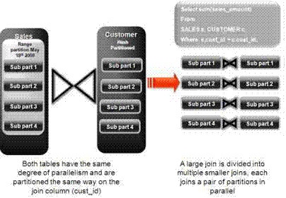
A major performance benefit of hash partitioning is partition-wise joins. Partition-wise joins reduce query response time by minimizing the amount of data exchanged among parallel execution servers when joins execute in parallel. This significantly reduces response time and improves both CPU and memory resource usage. In a clustered data warehouse, this significantly reduces response times by limiting the data traffic over the interconnect (IPC), which is the key to achieving good scalability for massive join operations. Partition-wise joins can be full or partial, depending on the partitioning scheme of the tables to be joined.
As illustrated in Figure 2-2, a full partition-wise join divides a join between two large tables into multiple smaller joins. Each smaller join, performs a joins on a pair of partitions, one for each of the tables being joined. For the optimizer to choose the full partition-wise join method, both tables must be equi-partitioned on their join keys. That is, they have to be partitioned on the same column with the same partitioning method. Parallel execution of a full partition-wise join is similar to its serial execution, except that instead of joining one partition pair at a time, multiple partition pairs are joined in parallel by multiple parallel query servers. The number of partitions joined in parallel is determined by the Degree of Parallelism (DOP).
Figure 2-2 Partitioning for Join Performance
Recommendations: Number of Hash Partitions
To ensure that the data gets evenly distributed among the hash partitions it is highly recommended that the number of hash partitions is a power of 2 (for example, 2, 4, 8, and so on). A good rule of thumb to follow when deciding the number of hash partitions a table should have is 2 X # of CPUs rounded to up to the nearest power of 2.
If your system has 12 CPUs, then 32 would be a good number of hash partitions. On a clustered system the same rules apply. If you have 3 nodes each with 4 CPUs, then 32 would still be a good number of hash partitions. However, ensure that each hash partition is at least 16MB. Many small partitions do not have efficient scan rates with parallel query. Consequently, if using the number of CPUs makes the size of the hash partitions too small, use the number of Oracle RAC nodes in the environment (rounded to the nearest power of 2) instead.
Parallel Execution enables a database task to be parallelized or divided into smaller units of work, thus allowing multiple processes to work concurrently. By using parallelism, a terabyte of data can be scanned and processed in minutes or less, not hours or days.
Figure 2-3 illustrates the parallel execution of a full partition-wise join between two tables, Sales and Customers. Both tables have the same degree of parallelism and the same number of partitions. They are range partitioned on a date field and sub partitioned by hash on the cust_id field. As illustrated in the picture, each partition pair is read from the database and joined directly.
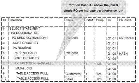
There is no data redistribution necessary, thus minimizing IPC communication, especially across nodes. Figure 2-3 shows the execution plan you would see for this join.
Figure 2-3 Parallel Execution of a Full Partition-Wise Join Between Two Tables
To ensure that you get optimal performance when executing a partition-wise join in parallel, use the degree of parallelism as a multiple of the number of partitions. The number of partitions should be multiple of the number of cores. To get best performance use degree of parallelism that is the same as the number of partitions to be processed in a query (this should be equal to number of CPU cores).
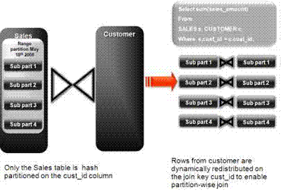
What happens if only one table that you are joining is partitioned? In this case the optimizer could pick a partial partition-wise join. Unlike full partition-wise joins, partial partition-wise joins can be applied if only one table is partitioned on the join key. Hence, partial partition-wise joins are more common than full partition-wise joins. To execute a partial partition-wise join, Oracle Database dynamically repartitions the other table based on the partitioning strategy of the partitioned table.
After the other table is repartitioned, the execution is similar to a full partition-wise join. The redistribution operation involves exchanging rows between parallel execution servers. This operation leads to interconnect traffic in Oracle RAC environments, since data must be repartitioned across node boundaries.
Figure 2-4 illustrates a partial partition-wise join. It uses the same example as in Figure 2-3, except that the customer table is not partitioned. Before the join operation is executed, the rows from the customers table are dynamically redistributed on the join key.
Parallel query is the most commonly used parallel execution feature in Oracle Database. Parallel execution can significantly reduce the elapsed time for large queries. To enable parallelization for an entire session, execute the following statement.
alter session enable parallel query;
Data Manipulation Language (DML) operations such as INSERT, UPDATE, and DELETE can be parallelized by Oracle Database. Parallel execution can speed up large DML operations and is particularly advantageous in data warehousing environments. To enable parallelization of DML statements, execute the following statement.
alter session enable parallel dml;
When you issue a DML statement such as an INSERT, UPDATE, or DELETE, Oracle Database applies a set of rules to determine whether that statement can be parallelized. The rules vary depending on whether the statement is a DML INSERT statement, or a DML UPDATE or DELETE statement.
The following rules apply when determining how to parallelize DML UPDATE and DELETE statements:
Oracle Database can parallelize UPDATE and DELETE statements on partitioned tables, but only when multiple partitions are involved.
You cannot parallelize UPDATE or DELETE operations on a nonpartitioned table or when such operations affect only a single partition.
The following rules apply when determining how to parallelize DML INSERT statements:
Standard INSERT statements using a VALUES clause cannot be parallelized.
Oracle Database can parallelize only INSERT . . . SELECT . . . FROM statements.
The setting of parallelism for a table influences the optimizer. Consequently, when using parallel query, also enable parallelism at the table level by issuing the following statement.
alter table <table_name> parallel 32;
|
Copyright © 2011, 2012, Oracle and/or its affiliates. All rights reserved. Legal Notices |
|