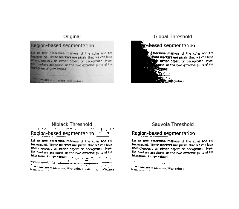
Niblack and Sauvola thresholds are local thresholding techniques that are useful for images where the background is not uniform, especially for text recognition [1], [2]. Instead of calculating a single global threshold for the entire image, several thresholds are calculated for every pixel by using specific formulae that take into account the mean and standard deviation of the local neighborhood (defined by a window centered around the pixel).
Here, we binarize an image using these algorithms compare it to a common global thresholding technique. Parameter window_size determines the size of the window that contains the surrounding pixels.
| [1] | Niblack, W (1986), An introduction to Digital Image Processing, Prentice-Hall. |
| [2] | J. Sauvola and M. Pietikainen, “Adaptive document image binarization,” Pattern Recognition 33(2), pp. 225-236, 2000. DOI:10.1016/S0031-3203(99)00055-2 |

import matplotlib
import matplotlib.pyplot as plt

from skimage.data import page
from skimage.filters import (threshold_otsu, threshold_niblack,
                             threshold_sauvola)


matplotlib.rcParams['font.size'] = 9


image = page()
binary_global = image > threshold_otsu(image)

window_size = 25
thresh_niblack = threshold_niblack(image, window_size=window_size, k=0.8)
thresh_sauvola = threshold_sauvola(image, window_size=window_size)

binary_niblack = image > thresh_niblack
binary_sauvola = image > thresh_sauvola

plt.figure(figsize=(8, 7))
plt.subplot(2, 2, 1)
plt.imshow(image, cmap=plt.cm.gray)
plt.title('Original')
plt.axis('off')

plt.subplot(2, 2, 2)
plt.title('Global Threshold')
plt.imshow(binary_global, cmap=plt.cm.gray)
plt.axis('off')

plt.subplot(2, 2, 3)
plt.imshow(binary_niblack, cmap=plt.cm.gray)
plt.title('Niblack Threshold')
plt.axis('off')

plt.subplot(2, 2, 4)
plt.imshow(binary_sauvola, cmap=plt.cm.gray)
plt.title('Sauvola Threshold')
plt.axis('off')

plt.show()
Total running time of the script: ( 0 minutes 0.171 seconds)