numpy.ma.polyfit
- numpy.ma.polyfit(x, y, deg, rcond=None, full=False, w=None, cov=False)[source]
Least squares polynomial fit.
Fit a polynomial p(x) = p[0] * x**deg + ... + p[deg] of degree deg to points (x, y). Returns a vector of coefficients p that minimises the squared error.
Parameters: x : array_like, shape (M,)
x-coordinates of the M sample points (x[i], y[i]).
y : array_like, shape (M,) or (M, K)
y-coordinates of the sample points. Several data sets of sample points sharing the same x-coordinates can be fitted at once by passing in a 2D-array that contains one dataset per column.
deg : int
Degree of the fitting polynomial
rcond : float, optional
Relative condition number of the fit. Singular values smaller than this relative to the largest singular value will be ignored. The default value is len(x)*eps, where eps is the relative precision of the float type, about 2e-16 in most cases.
full : bool, optional
Switch determining nature of return value. When it is False (the default) just the coefficients are returned, when True diagnostic information from the singular value decomposition is also returned.
w : array_like, shape (M,), optional
Weights to apply to the y-coordinates of the sample points. For gaussian uncertainties, use 1/sigma (not 1/sigma**2).
cov : bool, optional
Return the estimate and the covariance matrix of the estimate If full is True, then cov is not returned.
Returns: p : ndarray, shape (deg + 1,) or (deg + 1, K)
Polynomial coefficients, highest power first. If y was 2-D, the coefficients for k-th data set are in p[:,k].
residuals, rank, singular_values, rcond
Present only if full = True. Residuals of the least-squares fit, the effective rank of the scaled Vandermonde coefficient matrix, its singular values, and the specified value of rcond. For more details, see linalg.lstsq.
V : ndarray, shape (M,M) or (M,M,K)
Present only if full = False and cov`=True. The covariance matrix of the polynomial coefficient estimates. The diagonal of this matrix are the variance estimates for each coefficient. If y is a 2-D array, then the covariance matrix for the `k-th data set are in V[:,:,k]
Warns: RankWarning
The rank of the coefficient matrix in the least-squares fit is deficient. The warning is only raised if full = False.
The warnings can be turned off by
>>> import warnings
>>> warnings.simplefilter('ignore', np.RankWarning)
See also
- polyval
- Compute polynomial values.
- linalg.lstsq
- Computes a least-squares fit.
- scipy.interpolate.UnivariateSpline
- Computes spline fits.
Notes
Any masked values in x is propagated in y, and vice-versa.
References
[R52] Wikipedia, “Curve fitting”, http://en.wikipedia.org/wiki/Curve_fitting [R53] Wikipedia, “Polynomial interpolation”, http://en.wikipedia.org/wiki/Polynomial_interpolation Examples
>>> x = np.array([0.0, 1.0, 2.0, 3.0,  4.0,  5.0])
>>> y = np.array([0.0, 0.8, 0.9, 0.1, -0.8, -1.0])
>>> z = np.polyfit(x, y, 3)
>>> z
array([ 0.08703704, -0.81349206,  1.69312169, -0.03968254])
It is convenient to use poly1d objects for dealing with polynomials:
>>> p = np.poly1d(z)
>>> p(0.5)
0.6143849206349179
>>> p(3.5)
-0.34732142857143039
>>> p(10)
22.579365079365115
High-order polynomials may oscillate wildly:
>>> p30 = np.poly1d(np.polyfit(x, y, 30))
/... RankWarning: Polyfit may be poorly conditioned...
>>> p30(4)
-0.80000000000000204
>>> p30(5)
-0.99999999999999445
>>> p30(4.5)
-0.10547061179440398
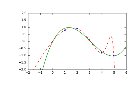
Illustration:
>>> import matplotlib.pyplot as plt
>>> xp = np.linspace(-2, 6, 100)
>>> _ = plt.plot(x, y, '.', xp, p(xp), '-', xp, p30(xp), '--')
>>> plt.ylim(-2,2)
(-2, 2)
>>> plt.show()
(Source code, png, pdf)
