
statsmodels.tsa.statespace.sarimax.SARIMAX
-
class
statsmodels.tsa.statespace.sarimax.SARIMAX(endog, exog=None, order=(1, 0, 0), seasonal_order=(0, 0, 0, 0), trend=None, measurement_error=False, time_varying_regression=False, mle_regression=True, simple_differencing=False, enforce_stationarity=True, enforce_invertibility=True, hamilton_representation=False, **kwargs)[source]¶ Seasonal AutoRegressive Integrated Moving Average with eXogenous regressors model
Parameters: endog : array_like
The observed time-series process

exog : array_like, optional
Array of exogenous regressors, shaped nobs x k.
order : iterable or iterable of iterables, optional
The (p,d,q) order of the model for the number of AR parameters, differences, and MA parameters. d must be an integer indicating the integration order of the process, while p and q may either be an integers indicating the AR and MA orders (so that all lags up to those orders are included) or else iterables giving specific AR and / or MA lags to include. Default is an AR(1) model: (1,0,0).
seasonal_order : iterable, optional
The (P,D,Q,s) order of the seasonal component of the model for the AR parameters, differences, MA parameters, and periodicity. d must be an integer indicating the integration order of the process, while p and q may either be an integers indicating the AR and MA orders (so that all lags up to those orders are included) or else iterables giving specific AR and / or MA lags to include. s is an integer giving the periodicity (number of periods in season), often it is 4 for quarterly data or 12 for monthly data. Default is no seasonal effect.
trend : str{‘n’,’c’,’t’,’ct’} or iterable, optional
Parameter controlling the deterministic trend polynomial
 .
Can be specified as a string where ‘c’ indicates a constant (i.e. a
degree zero component of the trend polynomial), ‘t’ indicates a
linear trend with time, and ‘ct’ is both. Can also be specified as an
iterable defining the polynomial as in numpy.poly1d, where
[1,1,0,1] would denote
.
Can be specified as a string where ‘c’ indicates a constant (i.e. a
degree zero component of the trend polynomial), ‘t’ indicates a
linear trend with time, and ‘ct’ is both. Can also be specified as an
iterable defining the polynomial as in numpy.poly1d, where
[1,1,0,1] would denote  . Default is to not
include a trend component.
. Default is to not
include a trend component.measurement_error : boolean, optional
Whether or not to assume the endogenous observations endog were measured with error. Default is False.
time_varying_regression : boolean, optional
Used when an explanatory variables, exog, are provided provided to select whether or not coefficients on the exogenous regressors are allowed to vary over time. Default is False.
mle_regression : boolean, optional
Whether or not to use estimate the regression coefficients for the exogenous variables as part of maximum likelihood estimation or through the Kalman filter (i.e. recursive least squares). If time_varying_regression is True, this must be set to False. Default is True.
simple_differencing : boolean, optional
Whether or not to use partially conditional maximum likelihood estimation. If True, differencing is performed prior to estimation, which discards the first
 initial rows but reuslts in a
smaller state-space formulation. If False, the full SARIMAX model is
put in state-space form so that all datapoints can be used in
estimation. Default is False.
initial rows but reuslts in a
smaller state-space formulation. If False, the full SARIMAX model is
put in state-space form so that all datapoints can be used in
estimation. Default is False.enforce_stationarity : boolean, optional
Whether or not to transform the AR parameters to enforce stationarity in the autoregressive component of the model. Default is True.
enforce_invertibility : boolean, optional
Whether or not to transform the MA parameters to enforce invertibility in the moving average component of the model. Default is True.
hamilton_representation : boolean, optional
Whether or not to use the Hamilton representation of an ARMA process (if True) or the Harvey representation (if False). Default is False.
**kwargs
Keyword arguments may be used to provide default values for state space matrices or for Kalman filtering options. See Representation, and KalmanFilter for more details.
Notes
The SARIMA model is specified
 .
.
In terms of a univariate structural model, this can be represented as
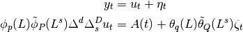
where
 is only applicable in the case of measurement error
(although it is also used in the case of a pure regression model, i.e. if
p=q=0).
is only applicable in the case of measurement error
(although it is also used in the case of a pure regression model, i.e. if
p=q=0).In terms of this model, regression with SARIMA errors can be represented easily as
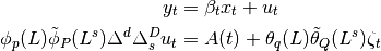
this model is the one used when exogenous regressors are provided.
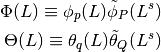
Note that the reduced form lag polynomials will be written as:
If mle_regression is True, regression coefficients are treated as additional parameters to be estimated via maximum likelihood. Otherwise they are included as part of the state with a diffuse initialization. In this case, however, with approximate diffuse initialization, results can be sensitive to the initial variance.
This class allows two different underlying representations of ARMA models as state space models: that of Hamilton and that of Harvey. Both are equivalent in the sense that they are analytical representations of the ARMA model, but the state vectors of each have different meanings. For this reason, maximum likelihood does not result in identical parameter estimates and even the same set of parameters will result in different loglikelihoods.
The Harvey representation is convenient because it allows integrating differencing into the state vector to allow using all observations for estimation.
In this implementation of differenced models, the Hamilton representation is not able to accomodate differencing in the state vector, so simple_differencing (which performs differencing prior to estimation so that the first d + sD observations are lost) must be used.
Many other packages use the Hamilton representation, so that tests against Stata and R require using it along with simple differencing (as Stata does).
Detailed information about state space models can be found in [R80]. Some specific references are:
- Chapter 3.4 describes ARMA and ARIMA models in state space form (using the Harvey representation), and gives references for basic seasonal models and models with a multiplicative form (for example the airline model). It also shows a state space model for a full ARIMA process (this is what is done here if simple_differencing=False).
- Chapter 3.6 describes estimating regression effects via the Kalman filter (this is performed if mle_regression is False), regression with time-varying coefficients, and regression with ARMA errors (recall from above that if regression effects are present, the model estimated by this class is regression with SARIMA errors).
- Chapter 8.4 describes the application of an ARMA model to an example dataset. A replication of this section is available in an example IPython notebook in the documentation.
References
[R80] (1, 2) Durbin, James, and Siem Jan Koopman. 2012. Time Series Analysis by State Space Methods: Second Edition. Oxford University Press. Attributes
measurement_error (boolean) Whether or not to assume the endogenous observations endog were measured with error. state_error (boolean) Whether or not the transition equation has an error component. mle_regression (boolean) Whether or not the regression coefficients for the exogenous variables were estimated via maximum likelihood estimation. state_regression (boolean) Whether or not the regression coefficients for the exogenous variables are included as elements of the state space and estimated via the Kalman filter. time_varying_regression (boolean) Whether or not coefficients on the exogenous regressors are allowed to vary over time. simple_differencing (boolean) Whether or not to use partially conditional maximum likelihood estimation. enforce_stationarity (boolean) Whether or not to transform the AR parameters to enforce stationarity in the autoregressive component of the model. enforce_invertibility (boolean) Whether or not to transform the MA parameters to enforce invertibility in the moving average component of the model. hamilton_representation (boolean) Whether or not to use the Hamilton representation of an ARMA process. trend (str{‘n’,’c’,’t’,’ct’} or iterable) Parameter controlling the deterministic trend polynomial . See the class parameter documentation for more information.polynomial_ar (array) Array containing autoregressive lag polynomial coefficients, ordered from lowest degree to highest. Initialized with ones, unless a coefficient is constrained to be zero (in which case it is zero). polynomial_ma (array) Array containing moving average lag polynomial coefficients, ordered from lowest degree to highest. Initialized with ones, unless a coefficient is constrained to be zero (in which case it is zero). polynomial_seasonal_ar (array) Array containing seasonal moving average lag polynomial coefficients, ordered from lowest degree to highest. Initialized with ones, unless a coefficient is constrained to be zero (in which case it is zero). polynomial_seasonal_ma (array) Array containing seasonal moving average lag polynomial coefficients, ordered from lowest degree to highest. Initialized with ones, unless a coefficient is constrained to be zero (in which case it is zero). polynomial_trend (array) Array containing trend polynomial coefficients, ordered from lowest degree to highest. Initialized with ones, unless a coefficient is constrained to be zero (in which case it is zero). k_ar (int) Highest autoregressive order in the model, zero-indexed. k_ar_params (int) Number of autoregressive parameters to be estimated. k_diff (int) Order of intergration. k_ma (int) Highest moving average order in the model, zero-indexed. k_ma_params (int) Number of moving average parameters to be estimated. seasonal_periods (int) Number of periods in a season. k_seasonal_ar (int) Highest seasonal autoregressive order in the model, zero-indexed. k_seasonal_ar_params (int) Number of seasonal autoregressive parameters to be estimated. k_seasonal_diff (int) Order of seasonal intergration. k_seasonal_ma (int) Highest seasonal moving average order in the model, zero-indexed. k_seasonal_ma_params (int) Number of seasonal moving average parameters to be estimated. k_trend (int) Order of the trend polynomial plus one (i.e. the constant polynomial would have k_trend=1). k_exog (int) Number of exogenous regressors. Methods
filter(params, **kwargs)fit([start_params, transformed, cov_type, ...])Fits the model by maximum likelihood via Kalman filter. from_formula(formula, data[, subset])Not implemented for state space models hessian(params, *args, **kwargs)Hessian matrix of the likelihood function, evaluated at the given impulse_responses(params[, steps, impulse, ...])Impulse response function information(params)Fisher information matrix of model initialize()Initialize the SARIMAX model. initialize_approximate_diffuse([variance])Initialize the statespace model with approximate diffuse values. initialize_known(initial_state, ...)Initialize the statespace model with known distribution for initial state. initialize_state([variance, complex_step])Initialize state and state covariance arrays in preparation for the Kalman filter. initialize_statespace(**kwargs)Initialize the state space representation initialize_stationary()Initialize the statespace model as stationary. loglike(params, *args, **kwargs)Loglikelihood evaluation loglikeobs(params[, transformed, complex_step])Loglikelihood evaluation observed_information_matrix(params[, ...])Observed information matrix opg_information_matrix(params[, ...])Outer product of gradients information matrix predict(params[, exog])After a model has been fit predict returns the fitted values. prepare_data()score(params, *args, **kwargs)Compute the score function at params. score_obs(params[, method, transformed, ...])Compute the score per observation, evaluated at params set_conserve_memory([conserve_memory])Set the memory conservation method set_filter_method([filter_method])Set the filtering method set_inversion_method([inversion_method])Set the inversion method set_smoother_output([smoother_output])Set the smoother output set_stability_method([stability_method])Set the numerical stability method simulate(params, nsimulations[, ...])Simulate a new time series following the state space model smooth(params, **kwargs)transform_jacobian(unconstrained[, ...])Jacobian matrix for the parameter transformation function transform_params(unconstrained)Transform unconstrained parameters used by the optimizer to constrained parameters used in likelihood evaluation. untransform_params(constrained)Transform constrained parameters used in likelihood evaluation update(params[, transformed, complex_step])Update the parameters of the model Methods
filter(params, **kwargs)fit([start_params, transformed, cov_type, ...])Fits the model by maximum likelihood via Kalman filter. from_formula(formula, data[, subset])Not implemented for state space models hessian(params, *args, **kwargs)Hessian matrix of the likelihood function, evaluated at the given impulse_responses(params[, steps, impulse, ...])Impulse response function information(params)Fisher information matrix of model initialize()Initialize the SARIMAX model. initialize_approximate_diffuse([variance])Initialize the statespace model with approximate diffuse values. initialize_known(initial_state, ...)Initialize the statespace model with known distribution for initial state. initialize_state([variance, complex_step])Initialize state and state covariance arrays in preparation for the Kalman filter. initialize_statespace(**kwargs)Initialize the state space representation initialize_stationary()Initialize the statespace model as stationary. loglike(params, *args, **kwargs)Loglikelihood evaluation loglikeobs(params[, transformed, complex_step])Loglikelihood evaluation observed_information_matrix(params[, ...])Observed information matrix opg_information_matrix(params[, ...])Outer product of gradients information matrix predict(params[, exog])After a model has been fit predict returns the fitted values. prepare_data()score(params, *args, **kwargs)Compute the score function at params. score_obs(params[, method, transformed, ...])Compute the score per observation, evaluated at params set_conserve_memory([conserve_memory])Set the memory conservation method set_filter_method([filter_method])Set the filtering method set_inversion_method([inversion_method])Set the inversion method set_smoother_output([smoother_output])Set the smoother output set_stability_method([stability_method])Set the numerical stability method simulate(params, nsimulations[, ...])Simulate a new time series following the state space model smooth(params, **kwargs)transform_jacobian(unconstrained[, ...])Jacobian matrix for the parameter transformation function transform_params(unconstrained)Transform unconstrained parameters used by the optimizer to constrained parameters used in likelihood evaluation. untransform_params(constrained)Transform constrained parameters used in likelihood evaluation update(params[, transformed, complex_step])Update the parameters of the model Attributes
endog_namesNames of endogenous variables exog_namesinitial_designInitial design matrix initial_selectionInitial selection matrix initial_state_interceptInitial state intercept vector initial_transitionInitial transition matrix initial_varianceinitializationloglikelihood_burnmodel_latex_namesThe latex names of all possible model parameters. model_namesThe plain text names of all possible model parameters. model_ordersThe orders of each of the polynomials in the model. param_namesList of human readable parameter names (for parameters actually included in the model). param_termsList of parameters actually included in the model, in sorted order. params_completestart_paramsStarting parameters for maximum likelihood estimation tolerance