statsmodels.tsa.filters.bk_filter.bkfilter

statsmodels.tsa.filters.bk_filter.bkfilter(X, low=6, high=32, K=12)

Baxter-King bandpass filter

Parameters:

X : array-like

A 1 or 2d ndarray. If 2d, variables are assumed to be in columns.

low : float

Minimum period for oscillations, ie., Baxter and King suggest that the Burns-Mitchell U.S. business cycle has 6 for quarterly data and 1.5 for annual data.

high : float

Maximum period for oscillations BK suggest that the U.S. business cycle has 32 for quarterly data and 8 for annual data.

K : int

Lead-lag length of the filter. Baxter and King propose a truncation length of 12 for quarterly data and 3 for annual data.

Returns:

Y : array

Cyclical component of X

See also

statsmodels.tsa.filters.cf_filter.cffilter, statsmodels.tsa.filters.hp_filter.hpfilter, statsmodels.tsa.seasonal.seasonal_decompose

Notes

Returns a centered weighted moving average of the original series. Where the weights a[j] are computed

a[j] = b[j] + theta, for j = 0, +/-1, +/-2, ... +/- K
b[0] = (omega_2 - omega_1)/pi
b[j] = 1/(pi*j)(sin(omega_2*j)-sin(omega_1*j), for j = +/-1, +/-2,...

and theta is a normalizing constant

theta = -sum(b)/(2K+1)

References

Baxter, M. and R. G. King. “Measuring Business Cycles: Approximate

Band-Pass Filters for Economic Time Series.” Review of Economics and Statistics, 1999, 81(4), 575-593.

Examples

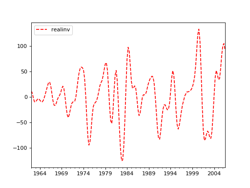
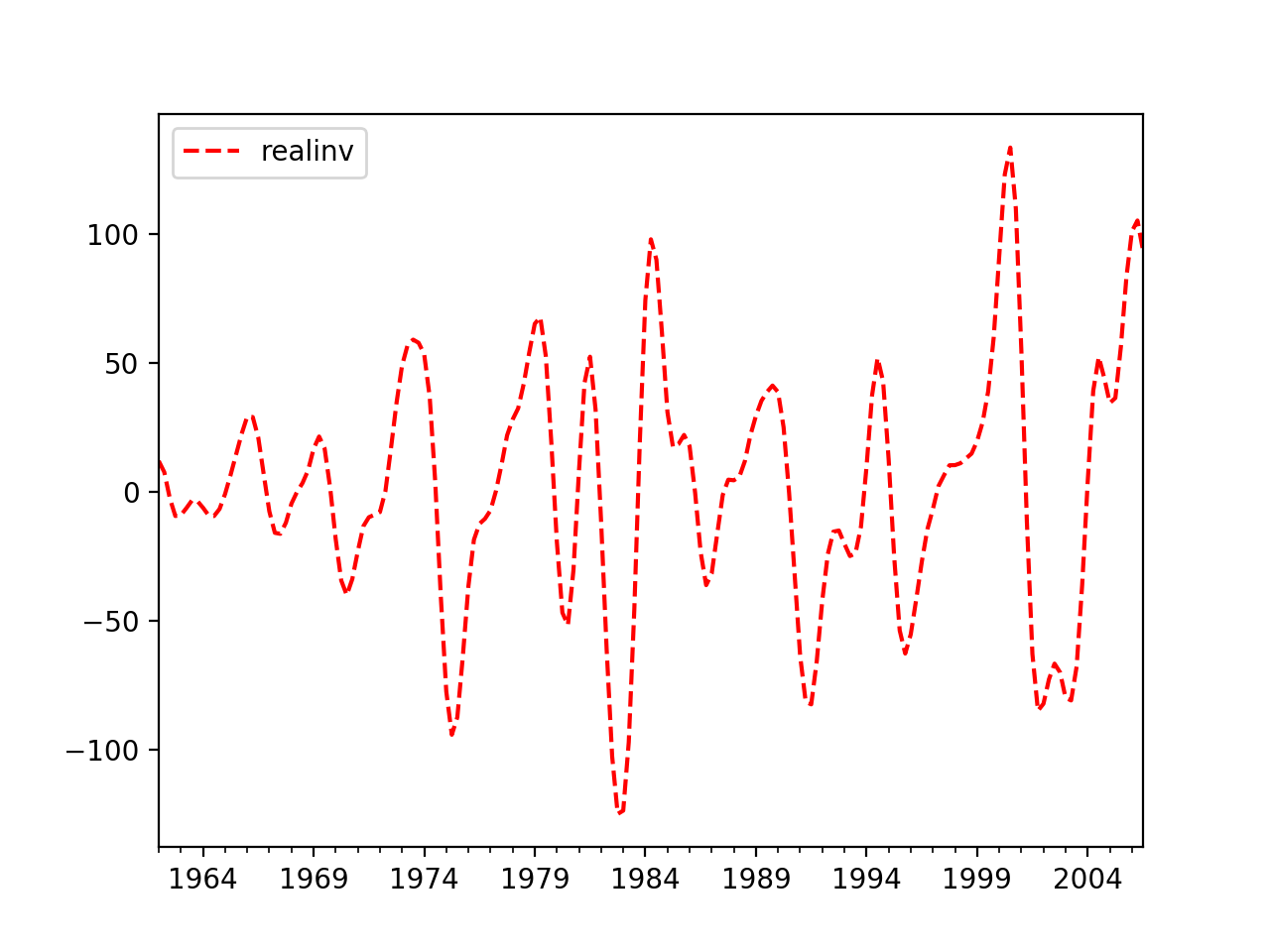
>>> import statsmodels.api as sm
>>> import pandas as pd
>>> dta = sm.datasets.macrodata.load_pandas().data
>>> index = pd.DatetimeIndex(start='1959Q1', end='2009Q4', freq='Q')
>>> dta.set_index(index, inplace=True)

>>> cycles = sm.tsa.filters.bkfilter(dta[['realinv']], 6, 24, 12)

>>> import matplotlib.pyplot as plt
>>> fig, ax = plt.subplots()
>>> cycles.plot(ax=ax, style=['r--', 'b-'])
>>> plt.show()

(Source code, png, hires.png, pdf)