Plotting Learning Curves

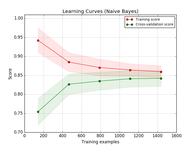
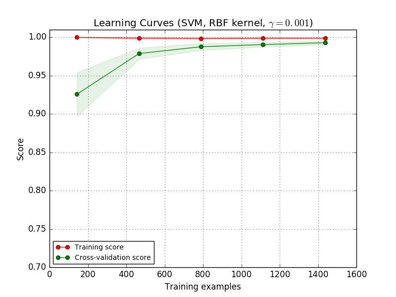
On the left side the learning curve of a naive Bayes classifier is shown for the digits dataset. Note that the training score and the cross-validation score are both not very good at the end. However, the shape of the curve can be found in more complex datasets very often: the training score is very high at the beginning and decreases and the cross-validation score is very low at the beginning and increases. On the right side we see the learning curve of an SVM with RBF kernel. We can see clearly that the training score is still around the maximum and the validation score could be increased with more training samples.

• 
• 

print(__doc__)

import numpy as np
import matplotlib.pyplot as plt
from sklearn.naive_bayes import GaussianNB
from sklearn.svm import SVC
from sklearn.datasets import load_digits
from sklearn.model_selection import learning_curve
from sklearn.model_selection import ShuffleSplit


def plot_learning_curve(estimator, title, X, y, ylim=None, cv=None,
                        n_jobs=1, train_sizes=np.linspace(.1, 1.0, 5)):
    """
    Generate a simple plot of the test and training learning curve.

    Parameters
    ----------
    estimator : object type that implements the "fit" and "predict" methods
        An object of that type which is cloned for each validation.

    title : string
        Title for the chart.

    X : array-like, shape (n_samples, n_features)
        Training vector, where n_samples is the number of samples and
        n_features is the number of features.

    y : array-like, shape (n_samples) or (n_samples, n_features), optional
        Target relative to X for classification or regression;
        None for unsupervised learning.

    ylim : tuple, shape (ymin, ymax), optional
        Defines minimum and maximum yvalues plotted.

    cv : int, cross-validation generator or an iterable, optional
        Determines the cross-validation splitting strategy.
        Possible inputs for cv are:
          - None, to use the default 3-fold cross-validation,
          - integer, to specify the number of folds.
          - An object to be used as a cross-validation generator.
          - An iterable yielding train/test splits.

        For integer/None inputs, if ``y`` is binary or multiclass,
        :class:`StratifiedKFold` used. If the estimator is not a classifier
        or if ``y`` is neither binary nor multiclass, :class:`KFold` is used.

        Refer :ref:`User Guide <cross_validation>` for the various
        cross-validators that can be used here.

    n_jobs : integer, optional
        Number of jobs to run in parallel (default 1).
    """
    plt.figure()
    plt.title(title)
    if ylim is not None:
        plt.ylim(*ylim)
    plt.xlabel("Training examples")
    plt.ylabel("Score")
    train_sizes, train_scores, test_scores = learning_curve(
        estimator, X, y, cv=cv, n_jobs=n_jobs, train_sizes=train_sizes)
    train_scores_mean = np.mean(train_scores, axis=1)
    train_scores_std = np.std(train_scores, axis=1)
    test_scores_mean = np.mean(test_scores, axis=1)
    test_scores_std = np.std(test_scores, axis=1)
    plt.grid()

    plt.fill_between(train_sizes, train_scores_mean - train_scores_std,
                     train_scores_mean + train_scores_std, alpha=0.1,
                     color="r")
    plt.fill_between(train_sizes, test_scores_mean - test_scores_std,
                     test_scores_mean + test_scores_std, alpha=0.1, color="g")
    plt.plot(train_sizes, train_scores_mean, 'o-', color="r",
             label="Training score")
    plt.plot(train_sizes, test_scores_mean, 'o-', color="g",
             label="Cross-validation score")

    plt.legend(loc="best")
    return plt


digits = load_digits()
X, y = digits.data, digits.target


title = "Learning Curves (Naive Bayes)"
# Cross validation with 100 iterations to get smoother mean test and train
# score curves, each time with 20% data randomly selected as a validation set.
cv = ShuffleSplit(n_splits=100, test_size=0.2, random_state=0)

estimator = GaussianNB()
plot_learning_curve(estimator, title, X, y, ylim=(0.7, 1.01), cv=cv, n_jobs=4)

title = "Learning Curves (SVM, RBF kernel, $\gamma=0.001$)"
# SVC is more expensive so we do a lower number of CV iterations:
cv = ShuffleSplit(n_splits=10, test_size=0.2, random_state=0)
estimator = SVC(gamma=0.001)
plot_learning_curve(estimator, title, X, y, (0.7, 1.01), cv=cv, n_jobs=4)

plt.show()

Total running time of the script: (0 minutes 10.943 seconds)

Download Python source code: plot_learning_curve.py

Download IPython notebook: plot_learning_curve.ipynb