Comparison of LDA and PCA 2D projection of Iris dataset¶

The Iris dataset represents 3 kind of Iris flowers (Setosa, Versicolour and Virginica) with 4 attributes: sepal length, sepal width, petal length and petal width.

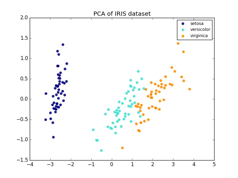
Principal Component Analysis (PCA) applied to this data identifies the combination of attributes (principal components, or directions in the feature space) that account for the most variance in the data. Here we plot the different samples on the 2 first principal components.

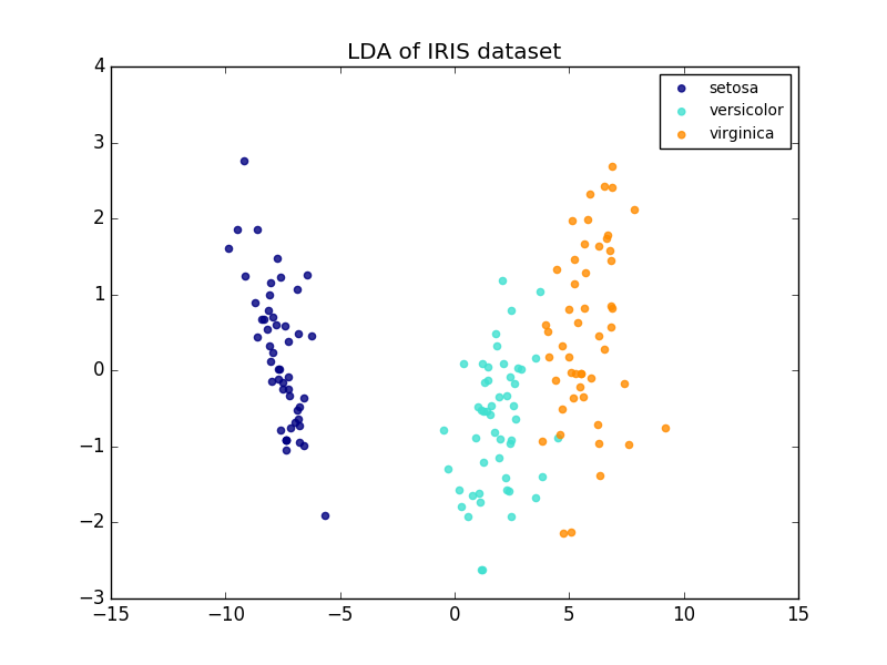
Linear Discriminant Analysis (LDA) tries to identify attributes that account for the most variance between classes. In particular, LDA, in contrast to PCA, is a supervised method, using known class labels.

Out:

explained variance ratio (first two components): [ 0.92461621  0.05301557]

print(__doc__)

import matplotlib.pyplot as plt

from sklearn import datasets
from sklearn.decomposition import PCA
from sklearn.discriminant_analysis import LinearDiscriminantAnalysis

iris = datasets.load_iris()

X = iris.data
y = iris.target
target_names = iris.target_names

pca = PCA(n_components=2)
X_r = pca.fit(X).transform(X)

lda = LinearDiscriminantAnalysis(n_components=2)
X_r2 = lda.fit(X, y).transform(X)

# Percentage of variance explained for each components
print('explained variance ratio (first two components): %s'
      % str(pca.explained_variance_ratio_))

plt.figure()
colors = ['navy', 'turquoise', 'darkorange']
lw = 2

for color, i, target_name in zip(colors, [0, 1, 2], target_names):
    plt.scatter(X_r[y == i, 0], X_r[y == i, 1], color=color, alpha=.8, lw=lw,
                label=target_name)
plt.legend(loc='best', shadow=False, scatterpoints=1)
plt.title('PCA of IRIS dataset')

plt.figure()
for color, i, target_name in zip(colors, [0, 1, 2], target_names):
    plt.scatter(X_r2[y == i, 0], X_r2[y == i, 1], alpha=.8, color=color,
                label=target_name)
plt.legend(loc='best', shadow=False, scatterpoints=1)
plt.title('LDA of IRIS dataset')

plt.show()

Total running time of the script: (0 minutes 0.180 seconds)

Download Python source code: plot_pca_vs_lda.py

Download IPython notebook: plot_pca_vs_lda.ipynb