Docs for 0.13.1
All versions

GLCM Texture Features¶

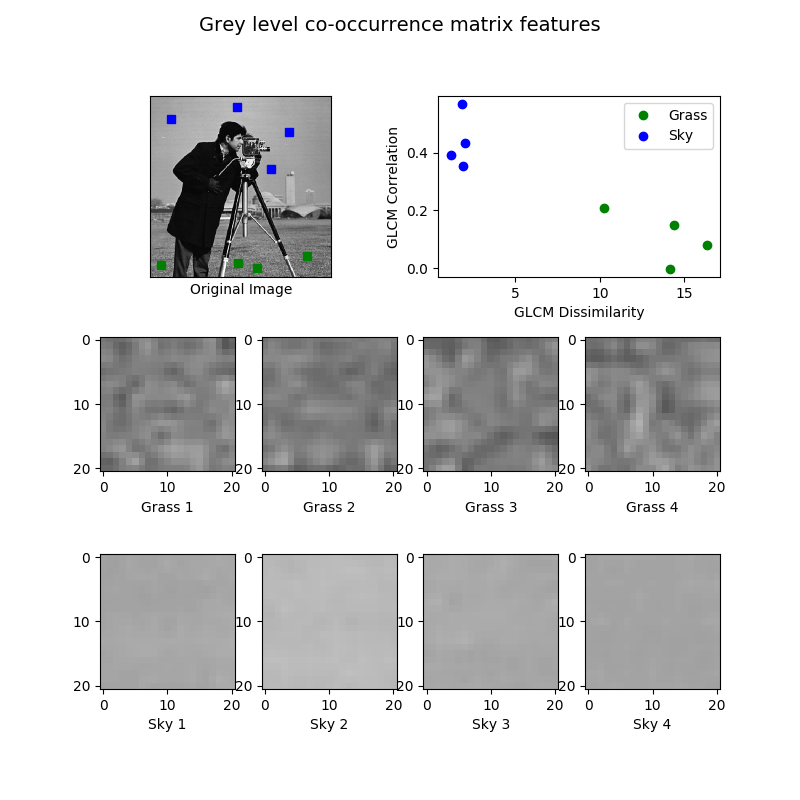
This example illustrates texture classification using grey level co-occurrence matrices (GLCMs). A GLCM is a histogram of co-occurring greyscale values at a given offset over an image.

In this example, samples of two different textures are extracted from an image: grassy areas and sky areas. For each patch, a GLCM with a horizontal offset of 5 is computed. Next, two features of the GLCM matrices are computed: dissimilarity and correlation. These are plotted to illustrate that the classes form clusters in feature space.

In a typical classification problem, the final step (not included in this example) would be to train a classifier, such as logistic regression, to label image patches from new images.

../../_images/sphx_glr_plot_glcm_001.png

import matplotlib.pyplot as plt

from skimage.feature import greycomatrix, greycoprops
from skimage import data


PATCH_SIZE = 21

# open the camera image
image = data.camera()

# select some patches from grassy areas of the image
grass_locations = [(474, 291), (440, 433), (466, 18), (462, 236)]
grass_patches = []
for loc in grass_locations:
    grass_patches.append(image[loc[0]:loc[0] + PATCH_SIZE,
                               loc[1]:loc[1] + PATCH_SIZE])

# select some patches from sky areas of the image
sky_locations = [(54, 48), (21, 233), (90, 380), (195, 330)]
sky_patches = []
for loc in sky_locations:
    sky_patches.append(image[loc[0]:loc[0] + PATCH_SIZE,
                             loc[1]:loc[1] + PATCH_SIZE])

# compute some GLCM properties each patch
xs = []
ys = []
for patch in (grass_patches + sky_patches):
    glcm = greycomatrix(patch, [5], [0], 256, symmetric=True, normed=True)
    xs.append(greycoprops(glcm, 'dissimilarity')[0, 0])
    ys.append(greycoprops(glcm, 'correlation')[0, 0])

# create the figure
fig = plt.figure(figsize=(8, 8))

# display original image with locations of patches
ax = fig.add_subplot(3, 2, 1)
ax.imshow(image, cmap=plt.cm.gray, interpolation='nearest',
          vmin=0, vmax=255)
for (y, x) in grass_locations:
    ax.plot(x + PATCH_SIZE / 2, y + PATCH_SIZE / 2, 'gs')
for (y, x) in sky_locations:
    ax.plot(x + PATCH_SIZE / 2, y + PATCH_SIZE / 2, 'bs')
ax.set_xlabel('Original Image')
ax.set_xticks([])
ax.set_yticks([])
ax.axis('image')

# for each patch, plot (dissimilarity, correlation)
ax = fig.add_subplot(3, 2, 2)
ax.plot(xs[:len(grass_patches)], ys[:len(grass_patches)], 'go',
        label='Grass')
ax.plot(xs[len(grass_patches):], ys[len(grass_patches):], 'bo',
        label='Sky')
ax.set_xlabel('GLCM Dissimilarity')
ax.set_ylabel('GLCM Correlation')
ax.legend()

# display the image patches
for i, patch in enumerate(grass_patches):
    ax = fig.add_subplot(3, len(grass_patches), len(grass_patches)*1 + i + 1)
    ax.imshow(patch, cmap=plt.cm.gray, interpolation='nearest',
              vmin=0, vmax=255)
    ax.set_xlabel('Grass %d' % (i + 1))

for i, patch in enumerate(sky_patches):
    ax = fig.add_subplot(3, len(sky_patches), len(sky_patches)*2 + i + 1)
    ax.imshow(patch, cmap=plt.cm.gray, interpolation='nearest',
              vmin=0, vmax=255)
    ax.set_xlabel('Sky %d' % (i + 1))


# display the patches and plot
fig.suptitle('Grey level co-occurrence matrix features', fontsize=14)
plt.show()

Total running time of the script: ( 0 minutes 0.389 seconds)

Generated by Sphinx-Gallery